The current-driven internal kink mode: Rosenbluth, Dagazian, and Rutherford

← Previous Lecture Contents Next Lecture →

Lecture 24
The current-driven internal kink mode: Rosenbluth, Dagazian, and Rutherford

Overview

The Kruskal–Shafranov lecture showed that a periodic screw pinch becomes current-driven unstable when the edge safety factor falls below unity, while the external-kink lecture showed how that same instability survives when the whole column pushes against the vacuum region. The next question is what happens when the dangerous $q=1$ surface lies inside the plasma rather than at its edge. Rosenbluth, Dagazian, and Rutherford showed that the $m=1$ family is then exceptional: in the cylindrical tokamak limit its leading restoring term vanishes, a rigid core shift becomes possible, and the ideal eigenfunction develops the singular internal-kink structure that later became central to sawtooth theory.

Historical Perspective

Large-aspect-ratio tokamak theory translated Newcomb’s general screw-pinch language into the experimentally meaningful language of the safety factor $q(r)$ Shafranov (1966); Newcomb (1960). The cylindrical $m=1$ internal kink later became central to sawtooth theory. The decisive large-aspect-ratio calculation is due to Rosenbluth, Dagazian, and Rutherford, who showed that once a $q=1$ surface appears inside the plasma the minimizing displacement is a rigid core shift cut off across a narrow internal layer Rosenbluth et al. (1973). In this lecture we stay strictly within that cylindrical, large-aspect-ratio tokamak limit. Toroidal sideband coupling will be introduced later in the TAE chapter as a clean harmonic-coupling problem. Here we only preview its effect on the internal kink, without carrying out the full Bussac derivation.

24.1 Large-aspect-ratio reduction

Ordering. Take a tokamak of major radius $R_0$ and minor radius $a$ with

\epsilon \equiv \frac {r}{R_0}\ll 1, \qquad \frac {B_\theta }{B_z}\sim \epsilon , \qquad \beta \sim \epsilon ^2,

so that the guide field is approximately uniform,

B_z(r)\simeq B_0, \qquad B_0=\text {constant to leading order}.

This is the cylindrical tokamak limit, not the reversed-field-pinch limit of the appendix: the axial field remains large and nearly constant, while the poloidal field is smaller by one power of $\epsilon $. Write the axial wavenumber as

k_z=\frac {n}{R_0}, \qquad k_z r \ll 1,

and use the cylindrical safety factor

q(r)=\frac {rB_z}{R_0 B_\theta }. \tag{24.4}

Then

B_\theta (r)\simeq \frac {rB_0}{R_0 q(r)}.

The field-line factors. With (24.4),

F(r) = \frac {mB_\theta }{r}-k_zB_z = \frac {B_0}{R_0}\left (\frac {m}{q(r)}-n\right ), \tag{24.6}

F^\dagger (r) = k_zB_z+\frac {mB_\theta }{r} = \frac {B_0}{R_0}\left (n+\frac {m}{q(r)}\right ). \tag{24.7}

Also,

k_0^2r^2=m^2+\frac {n^2r^2}{R_0^2}=m^2+O(\epsilon ^2).

Only $F^2$ and $(F^\dagger )^2$ enter the radial energy, so nothing below depends on the sign convention for $k_z$. The choice above keeps the usual tokamak combination $n-m/q$ visible.

Large-aspect-ratio forms of $f$ and $g$. To leading order Eqs. (21.83) and (21.91) become

\begin{aligned}f(r) &= \frac {rF^2}{k_0^2} \approx \frac {B_0^2 r^3}{m^2R_0^2}\left (n-\frac {m}{q(r)}\right )^2, \\ g(r) &\approx \frac {B_0^2 r}{m^2R_0^2}(m^2-1) \left (n-\frac {m}{q(r)}\right )^2 + \frac {2n^2r^2}{m^2R_0^2}\muo p'(r).\end{aligned} \tag{24.9}

The first term in (24.10) is line bending and geometry; the second is the pressure drive already encoded locally by Suydam.

Large-aspect-ratio forms of $f$ and $g$ to next order. Let \[ \Delta (r)\equiv n-\frac {m}{q(r)}, \qquad \Sigma (r)\equiv n+\frac {m}{q(r)}, \qquad \delta (r)\equiv \frac {n^2r^2}{m^2R_0^2}\ll 1. \] Using \[ F=-\frac {B_0}{R_0}\Delta , \qquad F^\dagger =-\frac {B_0}{R_0}\Sigma , \qquad k_0^2=\frac {m^2}{r^2}\left (1+\delta \right ), \] one finds

\begin{aligned}f(r) &= \frac {B_0^2r^3}{m^2R_0^2}\Delta ^2 \left [ 1-\frac {n^2r^2}{m^2R_0^2} +O\!\left (\frac {r^4}{R_0^4}\right ) \right ], \\ g(r) &= \frac {B_0^2r}{m^2R_0^2}(m^2-1)\Delta ^2 +\frac {2n^2r^2}{m^2R_0^2}\muo p'(r) +\frac {n^2B_0^2r^3}{m^4R_0^4} \left ( 3n^2-\frac {2nm}{q(r)}-\frac {m^2}{q(r)^2} \right ) +O\!\left (\frac {r^4}{R_0^4}\muo p',\frac {r^5B_0^2}{R_0^6}\right ).\end{aligned} \tag{24.12}

For the internal kink with $m=n=1$, this reduces to

\begin{aligned}f_{11}(r) &= \frac {B_0^2r^3}{R_0^2} \left (1-\frac {1}{q}\right )^2 \left [ 1-\frac {r^2}{R_0^2} +O\!\left (\frac {r^4}{R_0^4}\right ) \right ], \\ g_{11}(r) &= \frac {2r^2}{R_0^2}\muo p'(r) + \frac {B_0^2r^3}{R_0^4} \left (1-\frac {1}{q(r)}\right ) \left (3+\frac {1}{q(r)}\right ) +O\!\left (\frac {r^4}{R_0^4}\muo p',\frac {r^5B_0^2}{R_0^6}\right ).\end{aligned} \tag{24.14}

24.2 Fixed-boundary internal modes

This chapter sits directly between the external-kink problem and the later toroidal calculations. The Kruskal–Shafranov lecture focused on the edge condition $q_a<1$, where the whole column can kink. The external-kink lecture kept that same global current-driven physics but emphasized the vacuum matching outside the plasma. Here the edge remains fixed and the instability is instead tied to an internal $q=1$ surface. The result is a different eigenfunction structure, but it is still the same current-driven $m=1$ family.

Why $\xi _a=0$ is imposed here. Throughout this lecture we stay in Newcomb’s fixed-boundary sector,

\xi _a\equiv \xi (a)=0.

So every instability discussed below is internal by construction. The edge is held fixed while the plasma tries to reorganize inside. If the minimizing mode requires $\xi _a\neq 0$, that mode belongs to the external problem treated in the next lecture, not to the present one.

Low-$\beta $ internal stability for $m\ge 2$. If the pressure term is small enough that the local Suydam test has already been passed, then

\frac {\delta W}{2\pi ^2 R_0/\muo } \approx \frac {B_0^2}{R_0^2} \int _0^a \left (n-\frac {m}{q}\right )^2 \left [ \frac {r^3}{m^2}|\xi '|^2+\frac {m^2-1}{m^2}r|\xi |^2 \right ]dr. \tag{24.16}

For $m\ge 2$ the integrand is manifestly positive. Thus the leading-order large-aspect-ratio tokamak is internally stable to those families.

The $m=1$ internal kink. For $m=1$ the explicit $g$ term vanishes at leading order and a nearly rigid core displacement becomes possible. This is the exceptional current-driven family isolated by Rosenbluth, Dagazian, and Rutherford. If

\[q_0<1<q_a,\]

there is a resonant surface $r_s<a$ satisfying $q(r_s)=1$. A highly effective outer trial function is

\xi (r)\approx \begin {cases} \xi _0, & 0<r<r_s,\\[0.3em] 0, & r>r_s, \end {cases}

with a narrow transition layer. Because it vanishes for $r>r_s$, it already satisfies the fixed-edge condition $\xi _a=0$. This top-hat structure is the cylindrical Rosenbluth–Dagazian–Rutherford result: in their linear theory the minimizing singular solution is constant for $r<r_s$ and zero for $r>r_s$, and the exact resolved inner-layer profile tends to the same step in the ideal limit Rosenbluth et al. (1973). Since the leading $O(\epsilon ^2)$ functional is degenerate, the next-order contribution sets the sign of the energy:

\delta W_{4,cyl} = \frac {2 \pi ^2 B_z^2}{\mu _0 R_0} \xi _0^2 n^2 \int _0^{r_s} \left [ r\left (\dd {\beta }{r}\right ) + \frac {r^2}{R_0^2} \left (1-\frac {1}{q}\right )\left (3+\frac {1}{q}\right ) \right ]r\,dr, \tag{24.19}

Equation (24.19) is the large-aspect-ratio cylindrical contribution obtained by Rosenbluth, Dagazian, and Rutherford Rosenbluth et al. (1973).

A short toroidal outlook. The cylinder is not the final word. In a torus, the same $m=1$ core shift is coupled by the $R=R_0+r\cos \theta $ variation of the equilibrium field to stable $m=0$ and $m=2$ sidebands. So the large-aspect-ratio $n=1$ internal-kink energy is better thought of schematically as

\delta W \;\sim \; \delta W_{4,\mathrm {cyl}} \;+\; \delta W_{\mathrm {tor}}, \tag{24.20}

where $\delta W_{4,\mathrm {cyl}}$ is the cylindrical next-order RDR term (24.19), while $\delta W_{\mathrm {tor}}$ is the sideband-generated toroidal correction.

For the true $n=1$ internal kink, Bussac et al. showed that the toroidal contribution is not merely a small decoration of the cylindrical one. Their large-aspect-ratio decomposition may be written schematically as

\delta W = W_0 \left [ \left (1-\frac {1}{n^2}\right )\hat {\delta W}_{4,\mathrm {cyl}} + \frac {1}{n^2}\hat {\delta W}_{\mathrm {tor}} \right ], \tag{24.21}

so for $n=1$ only the toroidal correction survives. In the standard circular, parabolic-profile model this gives

\delta W = \frac {2\pi ^2 B_0^2}{\mu _0 R_0}\,\xi _0^2\, \frac {3r_1^4}{R_0^2}(1-q_0) \left ( \frac {13}{144}-\hat {\beta }_{p1}^{\,2} \right ), \tag{24.22}

with

\hat {\beta }_{p1} \equiv \frac {4\mu _0}{r_1^2B_p^2(r_1)} \int _0^{r_1} p(r)\,r\,dr. \tag{24.23}

Thus the torus can stabilize the ideal internal kink at low pressure; the instability threshold in that model is

\hat {\beta }_{p1}>\frac {\sqrt {13}}{12}\approx 0.30. \tag{24.24}

That is the only toroidal moral needed here: unlike the cylinder, the torus can change the sign of the $n=1$ internal-kink energy through sideband coupling.

Tutorial

What is being compressed into one formula. Rosenbluth, Dagazian, and Rutherford analyze the cylindrical $m=1$ mode and explain why the minimizing displacement is a rigid core shift with a narrow singular layer at $q=1$ Rosenbluth et al. (1973). The logic below is still entirely cylindrical: it explains the top-hat trial function, the degeneracy of the leading-order energy, and the inertial resolution of the internal layer. Toroidal sidebands are deliberately left for later.

The $O(\epsilon ^2)$ cylindrical functional has no $|\xi |^2$ cost. Setting $m=n=1$ in (24.16) gives
$\frac {\delta W_2}{2\pi ^2 R_0/\muo } \approx \frac {B_0^2}{R_0^2} \int _0^a \left (1-\frac {1}{q}\right )^2 r^3 |\xi '|^2\,dr. \tag{24.25}$ The explicit $|\xi |^2$ term vanishes because $m^2-1=0$. Thus only the thin matching region near $q=1$ costs energy. This is the cylindrical degeneracy behind the Rosenbluth–Dagazian–Rutherford step function Rosenbluth et al. (1973).

A simple minimizing sequence. Take $q(r_s)=1$ and define
$\xi _\delta (r)= \begin {cases} \xi _0, & r<r_s-\delta /2,\\[0.3em] \xi _0\left (\dfrac {r_s+\delta /2-r}{\delta }\right ), & |r-r_s|<\delta /2,\\[0.8em] 0, & r>r_s+\delta /2. \end {cases} \tag{24.26}$ Near $r_s$, $1-\frac {1}{q(r)} \approx \left .\dd {}{r}\left (1-\frac {1}{q}\right )\right |_{r_s}(r-r_s) = \frac {s_1}{r_s}(r-r_s), \qquad s_1\equiv r_s q'(r_s),$ so in the layer, $\begin{aligned}\frac {\delta W_2}{2\pi ^2 R_0/\muo } &\approx \frac {B_0^2}{R_0^2} \int _{-\delta /2}^{\delta /2} \left (\frac {s_1 x}{r_s}\right )^2 r_s^3\left (\frac {\xi _0}{\delta }\right )^2 dx \nonumber \\ &= \frac {B_0^2}{R_0^2} \frac {s_1^2 r_s\xi _0^2}{12}\,\delta \longrightarrow 0 \qquad (\delta \to 0).\end{aligned} \tag{24.28}$
So the top-hat profile is not merely heuristic: it is the minimizing sequence of the $O(\epsilon ^2)$ problem, which is why Rosenbluth et al. can take the outer solution to be constant inside $r_s$ and zero outside Rosenbluth et al. (1973).

The exact resolved jump from the singular layer. A triangular ramp is enough to prove (24.28), but the ideal problem by itself has only an infimum, not a smooth minimizer, so one must retain the small inertial term that resolves the singular layer. Rosenbluth–Dagazian–Rutherford then obtain the exact layer profile. Let
$x\equiv r-r_s, \qquad k\cdot B \approx (k\cdot B)'_s x,$ so their layer equation reduces to $\frac {d}{dx} \left [ \left ( 4\pi \rho _s\gamma ^2+(k\cdot B)_s'^2 x^2 \right ) \frac {d\xi }{dx} \right ] =0. \tag{24.30}$ Integrating once gives $\frac {d\xi }{dx} = \frac {C}{4\pi \rho _s\gamma ^2+(k\cdot B)_s'^2 x^2},$ and imposing $\xi \to \xi _s \quad (x\to -\infty ), \qquad \xi \to 0 \quad (x\to +\infty ),$ fixes the constants. The result is $\xi (x) = \frac {\xi _s}{2} \left [ 1- \frac {2}{\pi } \tan ^{-1} \left ( \frac {(k\cdot B)'_s x}{\gamma (4\pi \rho _s)^{1/2}} \right ) \right ]. \tag{24.33}$ Equivalently, with $\Delta \equiv \frac {\gamma (4\pi \rho _s)^{1/2}}{(k\cdot B)'_s},$ Eq. (24.33) is the arctangent-smoothed top hat. As $\Delta \to 0$ it reduces to the same rigid core shift Rosenbluth et al. (1973).

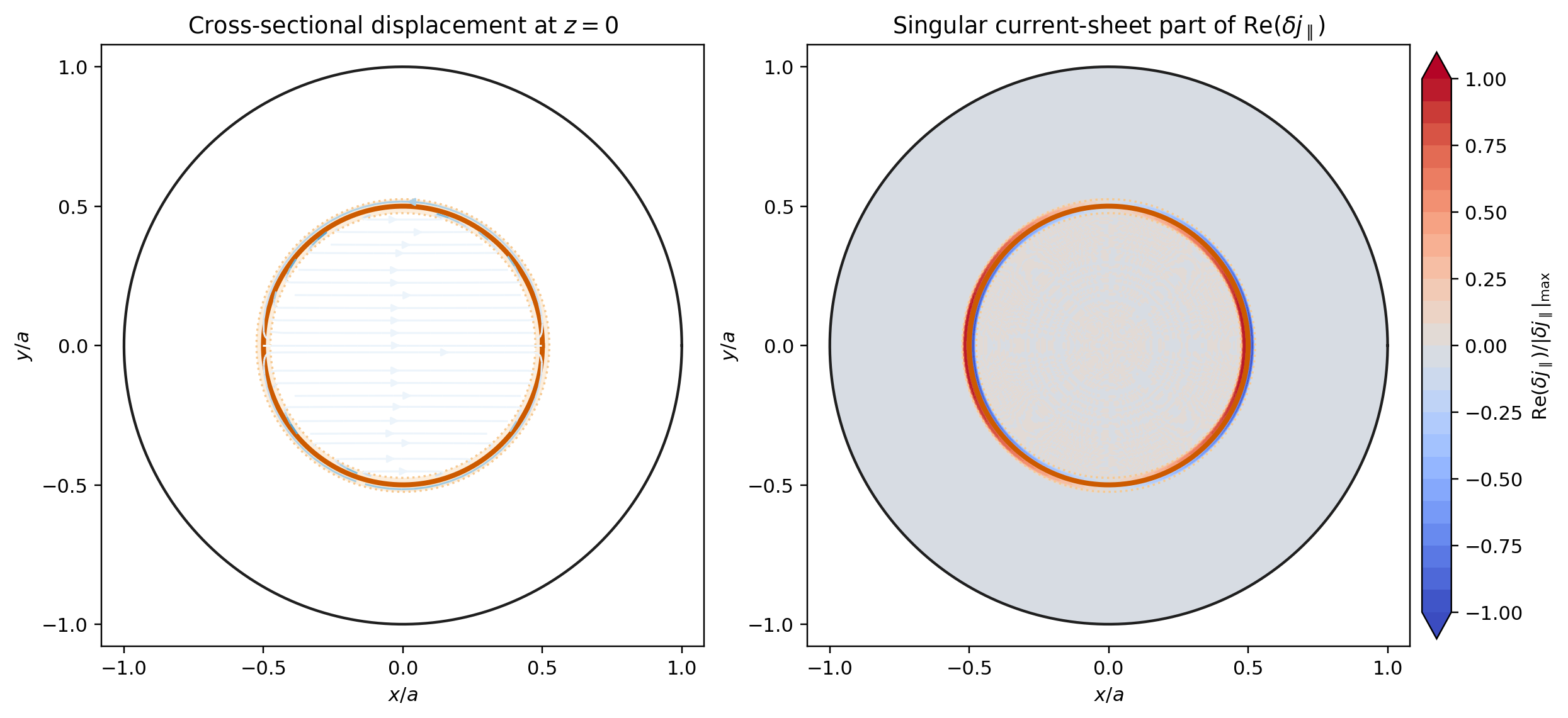
24.3 Cross-sectional structure and the nascent current sheet

The outer RDR eigenfunction is often summarized as a scalar radial amplitude $\xi _r(r)$, but the physical motion is not purely radial. Even in the cylindrical tokamak limit, incompressibility forces a large tangential displacement in the narrow $q=1$ layer. That same layer then produces a strongly peaked perturbed current density, which is the first hint that the ideal internal kink sits close to the resistive and tearing-mode physics of the next chapters.

Recover the transverse displacement. Take a single helical harmonic

\vect {\xi }(r,\theta ,z) = \Bigl [ \xi _r(r)\,\hat {\vect e}_r + \xi _\eta (r)\,\hat {\vect e}_\eta + \xi _\parallel (r)\,\bvec _0 \Bigr ] e^{i(m\theta +k_z z)}, \qquad k_z=\frac {n}{R_0}, \tag{24.35}

where the binormal direction is

\hat {\vect e}_\eta \equiv \frac {(m/r)\,\hat {\vect e}_\theta -k_z\,\hat {\vect e}_z} {\bigl [(m/r)^2+k_z^2\bigr ]^{1/2}}. \tag{24.36}

In the cylindrical tokamak limit $B_z\simeq B_0\gg B_\theta $, the parallel piece is smaller than the perpendicular motion, so at leading order the incompressibility constraint reduces to

\nabla \cdot \vect {\xi } = \frac {1}{r}\frac {d}{dr}(r\xi _r) + i\left [\left (\frac {m}{r}\right )^2+k_z^2\right ]^{1/2}\xi _\eta + O(\epsilon \,\xi _\parallel ) =0. \tag{24.37}

Thus

\xi _\eta (r) = i\, \frac {(r\xi _r)'} {\bigl (m^2+k_z^2r^2\bigr )^{1/2}}. \tag{24.38}

For the internal kink, $m=n=1$, so

\xi _\eta (r) = i\, \frac {(r\xi _r)'} {\bigl (1+k_z^2r^2\bigr )^{1/2}} \simeq i(r\xi _r)', \qquad k_z r\ll 1. \tag{24.39}

This is the same geometry used in the TAE chapter: the radial displacement fixes the tangential piece. On a $z=0$ cross section the physical motion is

\xi _r^{\rm phys}(r,\theta )=\xi _r(r)\cos \theta , \qquad \xi _\theta ^{\rm phys}(r,\theta )\simeq -(r\xi _r)'\sin \theta . \tag{24.40}

If $\xi _r=\xi _0$ is constant inside the $q=1$ surface, then $(r\xi _r)'=\xi _0$, and Eq. (24.40) becomes the uniform Cartesian shift \[ \xi _x=\xi _0, \qquad \xi _y=0. \] So the rigid core motion is not a slogan; it is the exact $m=1$ geometry of the incompressible core.

Why the current perturbation is singular. Now take

\vect {B}_0(r)=B_\theta (r)\,\hat {\vect e}_\theta +B_0\,\hat {\vect e}_z, \qquad B_\theta (r)\simeq \frac {rB_0}{R_0q(r)}, \qquad B_0\simeq \text {constant}. \tag{24.41}

The ideal magnetic perturbation is

\delta \vect {B} = \nabla \times (\vect {\xi }\times \vect {B}_0). \tag{24.42}

With $\xi _\parallel =0$ at leading order and (24.39), one finds

\delta B_r = i\left (k_zB_0+\frac {mB_\theta }{r}\right )\xi _r, \tag{24.43}

\delta B_\theta \simeq -k_zB_0\, \frac {(r\xi _r)'}{\sqrt {1+k_z^2r^2}} -\frac {d}{dr}\bigl (B_\theta \xi _r\bigr ), \tag{24.44}

while the leading pieces of $\delta B_z$ cancel because of incompressibility. Since $B_z\simeq B_0\gg B_\theta $, the perturbed parallel current is, to leading order,

\delta j_\parallel \simeq \delta j_z = \frac {1}{\mu _0 r}\frac {d}{dr}(r\delta B_\theta ) -\frac {i m}{\mu _0 r}\delta B_r. \tag{24.45}

The second term is smooth across the $q=1$ surface because it depends on $\xi _r$ itself. The singular behavior comes from the first term, which differentiates the layer structure in $(r\xi _r)'$. Schematically,

\delta j_{\parallel ,\mathrm {sheet}} \sim -\frac {B_0}{\mu _0R_0}\, \frac {d^2}{dr^2}(r\xi _r), \tag{24.46}

so the arctangent-smoothed top hat (24.33) produces a sharply localized current ribbon at the $q=1$ surface. In the ideal limit $\Delta \to 0$, that ribbon tends to a helical current sheet.

Figure 24.1: Cross-sectional view of the cylindrical $m=n=1$ internal kink, using the smoothed RDR layer profile with $\Delta =0.05a$ and a simple large-aspect-ratio $q(r)$ profile satisfying $q(r_1)=1$ at $r_1=0.5a$. The solid orange circle marks the $q=1$ surface, while the lighter dotted circles show the finite layer edges $r_1\pm \Delta /2$. Left: streamlines of the in-plane displacement field $(\xi _x,\xi _y)$, using exact rigid translation for $r<r_1-\Delta /2$, zero displacement for $r>r_1+\Delta /2$, and all of the turning confined to the finite layer. Right: the dominant singular part of $\mathrm {Re}(\delta j_\parallel )$, using that same compact-support layer to show the helical current ribbon concentrated at $q=1$. This is the ideal-MHD precursor of the resistive internal-kink and $m=1$ tearing physics discussed later.

Figure 24.1 is the geometric bridge from the ideal internal kink to the resistive chapters. The mode is not just a broad core translation. It also builds a very thin current ribbon at the $q=1$ surface. Once resistivity, electron inertia, or reconnection are allowed to matter, that current concentration is exactly where the ideal description must fail first. That is why the internal kink, the resistive internal kink, and the $m=1$ tearing mode are so closely linked.

24.4 Finite-length and line-tied descendants

The periodic cylindrical problem is only the first member of a larger family. Once the column has finite length and the ends are line tied, the eigenfunction can no longer be represented by a single axial Fourier factor with a resonant surface defined by $k\cdot B=0$. That was already one of the main lessons of the Kruskal–Shafranov lecture for the external kink. The same issue returns for the internal kink: line tying weakens the instability, changes the allowed axial structure, and removes the exact singularity of the periodic problem.

Finite-length screw pinch as the bridge problem. Ryutov, Cohen, and Pearlstein revisited the finite-length screw pinch and showed carefully why one cannot simply take an infinite-cylinder result and set $k_z=\pi /L$ by hand Ryutov et al. (2004). Hegna’s rotating-wall analysis made the same point from a neighboring direction: the end conditions and wall physics modify the admissible $m=1$ eigenfunctions before one ever asks about rotation or resistive-wall stabilization Hegna (2004). In that sense the line-tied current-driven kink is not a small correction to the periodic problem. It is a distinct boundary-value problem.

Internal kink in line-tied geometry. Huang, Zweibel, and Sovinec then asked the more specific question relevant here: what survives of the RDR internal kink when the screw pinch is line tied rather than periodic Huang et al. (2006)? Their main result is strikingly close to the cylindrical picture while still showing the importance of line tying. The fastest-growing line-tied $m=1$ internal kink still develops a strong radial gradient near the location corresponding to the periodic resonant surface, but the singular layer is broadened and the growth rate is reduced. As the system length $L$ increases, both the inner-layer thickness and the growth rate approach the periodic RDR values. In the small-twist limit $\epsilon \sim B_\phi /B_z$, they find a critical length $L_c\sim \epsilon ^{-3}$, and for $L\gtrsim L_c$ the line-tying correction to the layer thickness scales like $\epsilon ^{-1}(L_c/L)^{2.5}$ Huang et al. (2006). So line tying does not erase the internal-kink structure; it regularizes and weakens it.

Connection to coronal loops. The same mathematical problem also appears in the solar-coronal literature, where the ends of a flux rope are anchored in the dense photosphere rather than in conducting laboratory end plates. Velli, Hood, and Einaudi gave an early ideal-MHD treatment of line-tied coronal-loop kink modes and showed that the growth rate and eigenfunction depend strongly on loop length and field-line connectivity Velli et al. (1990). Lionello, Velli, Einaudi, and Mikić then followed the nonlinear evolution of line-tied coronal loops and showed how kink-driven current sheets and reconnection emerge once the ideal threshold is crossed Lionello et al. (1998). In that astrophysical language, the RDR internal kink becomes one member of the broader line-tied flux-rope instability family.

Connection to Wisconsin experiments and later computations. The Wisconsin line-tied screw-pinch program made these distinctions unusually concrete. Bergerson et al. directly observed the onset and saturation of the line-tied kink as the edge safety factor was driven below unity Bergerson et al. (2006), and later experiments separated ideal-wall, resistive-wall, and ferritic-wall effects in the same basic geometry Bergerson et al. (2008). Brookhart et al. then pushed the line-tied screw pinch into a zero-net-current regime where internal kink activity, reconnection, and turbulence all coexist Brookhart et al. (2015, 2017). Together with the computational treatments summarized by Schnack Schnack (2009), these works show that the line-tied internal kink is not just a solar or formal extension of RDR. It is also a laboratory problem with a direct bridge from ideal mode structure to nonlinear current-sheet formation.

Takeaways

The cylindrical $m=1$ internal kink is the cleanest example of an ideal-MHD mode whose minimizing sequence is almost discontinuous. The outer-region functional drives the core toward a rigid displacement inside the $q=1$ surface and near-zero displacement outside. The singular layer does not change that geometric picture; it resolves it. Once inertia is retained, the sharp top hat is replaced by the arctangent profile (24.33), which smooths the jump across a layer whose width shrinks with the growth rate. Finite-length and line-tied versions of the same problem retain that basic internal-kink geometry, but the end conditions weaken the instability, broaden the inner layer, and connect the RDR mode naturally to both coronal-loop theory and laboratory screw-pinch experiments.

Bibliography

V. D. Shafranov. Plasma equilibrium in a magnetic field. In M. A. Leontovich, editor, Reviews of Plasma Physics, volume 2, pages 103–151. Consultants Bureau, New York, 1966. Classic long review; includes the large-aspect-ratio treatment used for what is commonly called the Shafranov shift.

William A Newcomb. Hydromagnetic stability of a diffuse linear pinch. Annals of Physics, 10(2):232–267, 1960. doi:10.1016/0003-4916(60)90023-3.

Marshall N Rosenbluth, R Y Dagazian, and P H Rutherford. Nonlinear properties of the internal m = 1 kink instability in the cylindrical tokamak. The Physics of Fluids, 16(11):1894–1902, 1973. doi:10.1063/1.1694231.

D. D. Ryutov, R. H. Cohen, and L. D. Pearlstein. Stability of a finite-length screw pinch revisited. Physics of Plasmas, 11(10):4740–4752, 2004. ISSN 1070-664X. doi:10.1063/1.1781624.

C. C. Hegna. Stabilization of line tied resistive wall kink modes with rotating walls. Physics of Plasmas, 11(9):4230–4238, 2004. ISSN 1070-664X. doi:10.1063/1.1773777.

Yi-Min Huang, Ellen G. Zweibel, and Carl R. Sovinec. $m=1$ ideal internal kink modes in a line-tied screw pinch. Physics of Plasmas, 13(9):092102, 2006. doi:10.1063/1.2336506.

M. Velli, A. W. Hood, and G. Einaudi. Ideal kink instabilities in line-tied coronal loops: Growth rates and geometrical properties. The Astrophysical Journal, 350:428–436, 1990. doi:10.1086/168397.

R. Lionello, M. Velli, G. Einaudi, and Z. Miki\'c. Nonlinear magnetohydrodynamic evolution of line-tied coronal loops. The Astrophysical Journal, 494(2):840–850, 1998. doi:10.1086/305221.

W F Bergerson, C B Forest, G Fiksel, D A Hannum, R Kendrick, J S Sarff, and S Stambler. Onset and saturation of the kink instability in a current-carrying line-tied plasma. Physical Review Letters, 96(1):015004, 2006. doi:10.1103/physrevlett.96.015004.

W. F. Bergerson, D. A. Hannum, C. C. Hegna, R. D. Kendrick, J. S. Sarff, and C. B. Forest. Observation of resistive and ferritic wall modes in a line-tied pinch. Physical Review Letters, 101(23):235005, 2008. doi:10.1103/physrevlett.101.235005.

Matthew I. Brookhart, Aaron Stemo, Amanda Zuberbier, Ellen Zweibel, and Cary B. Forest. Instability, turbulence, and 3d magnetic reconnection in a line-tied, zero net current screw pinch. Physical Review Letters, 114(14):145001, 2015. doi:10.1103/physrevlett.114.145001.

Matthew I. Brookhart, Aaron Stemo, Roger Waleffe, and Cary B. Forest. Driving magnetic turbulence using flux ropes in a moderate guide field linear system. Journal of Plasma Physics, 83(6):905830604, 2017. doi:10.1017/s0022377817000794.

Dalton D. Schnack. Lectures in Magnetohydrodynamics: With an Appendix on Extended MHD, volume 780 of Lecture Notes in Physics. Springer, Berlin, Heidelberg, 2009. ISBN 9783642006876. doi:10.1007/978-3-642-00688-3.