External Kink Modes | Classic Problems in MHD

← Previous Lecture Contents Next Lecture →

Lecture 22
External Kink Modes

Overview

Only after the fixed-boundary problem has been cleared does it make sense to let the plasma edge move. In the external problem \(\xi _a\) is free, the vacuum and wall contribute to \(\delta W\), and instability occurs when the full plasma-plus-vacuum functional becomes negative for a mode with \(\xi _a\neq 0\).

Historical Perspective

The external kink is where Newcomb’s framework becomes practically important. The interior solution alone is not enough; one must also solve the vacuum problem and impose the wall boundary condition. That logic, already clear in cylindrical pinch theory, carried directly into tokamak design: internal profiles determine whether a regular plasma solution exists, while the vacuum region and conducting structures decide whether the boundary can bulge outward. That is one reason this sequence of lectures is so central historically.

22.1 Vacuum energy and the surface form of \(\delta W\)

Vacuum field. Let the plasma occupy \(0\le r\le a\), with vacuum in \(a<r<b\) and a perfectly conducting wall at \(r=b\). In vacuum,

\B _1 = -\grad \Phi , \qquad \lap \Phi = 0. \tag{22.1}

For a single helical harmonic,

\Phi (r,\theta ,z)=\phi (r)e^{i(m\theta +kz)}, \tag{22.2}

\frac {1}{r}\dd {}{r}\left (r\dd {\phi }{r}\right ) - \left (\frac {m^2}{r^2}+k^2\right )\phi =0. \tag{22.3}

The exact finite-\(k\) solutions are modified Bessel functions. For the large-aspect-ratio kink problem, however, \(|ka|\ll 1\), and it is more useful to display the long-wavelength form immediately:

\phi (r)=A r^{|m|}+B r^{-|m|}. \tag{22.4}

Wall condition. At a perfectly conducting wall,

B_{1r}(b)=-\pp {\Phi }{r}\bigg |_{r=b}=0 \qquad \Longrightarrow \qquad \phi '(b)=0. \tag{22.5}

Applying (22.5) to (22.4) gives

B = A\,b^{2|m|},

so that

\phi (r)=A\left (r^{|m|}+b^{2|m|}r^{-|m|}\right ).

Matching at the plasma boundary. At \(r=a\), ideal MHD requires

B_{1r}(a)= iF(a)\,\xi _a. \tag{22.8}

Since \(B_{1r}(a)=-\phi '(a)e^{i(m\theta +kz)}\),

-\phi '(a)=iF(a)\,\xi _a. \tag{22.9}

This fixes the constant \(A\), and evaluating the vacuum magnetic energy then produces a pure boundary term,

\delta W_v = \frac {\pi }{\muo }\,\frac {a^2F^2(a)}{|m|}\,\Lambda _m\,|\xi _a|^2, \tag{22.10}

where

\Lambda _m = \frac {1+\alpha _m}{1-\alpha _m}, \qquad \alpha _m\equiv \left (\frac {a}{b}\right )^{2|m|}. \tag{22.11}

The no-wall limit is \(\Lambda _m\rightarrow 1\).

Full reduced functional. Including the plasma term (21.92), the total energy is

\frac {\delta W}{2\pi ^2 R_0/\muo } = \int _0^a\left (f|\xi '|^2+g|\xi |^2\right )dr + \left [ \left (\frac {FF^\dagger }{k_0^2}\right )_{r=a} + \frac {a^2F^2(a)}{|m|}\Lambda _m \right ]|\xi _a|^2. \tag{22.12}

This is the master expression for the external ideal problem.

22.2 From the internal solution to the surface energy

What is assumed at this stage. At this point the local pressure-driven tests of Lecture 23 have been passed and the fixed-boundary internal problem of Lecture 24 has no unstable mode. One now reopens the variational problem by allowing the edge displacement \(\xi _a\) to be nonzero and by keeping the vacuum term in (22.12).

Convert the bulk term to a boundary term. Starting from

I\equiv \int _0^a\left (f|\xi '|^2+g|\xi |^2\right )dr,

use (21.99) in the form \(g\xi =(f\xi ')'\):

I = \int _0^a \left (f|\xi '|^2+(f\xi ')'\xi ^*\right )dr = \left [f\,\xi '\,\xi ^*\right ]_0^a .

Regularity makes the \(r=0\) term vanish, so

\int _0^a\left (f|\xi '|^2+g|\xi |^2\right )dr = f(a)\,\xi _a'\,\xi _a^*. \tag{22.15}

Substituting (22.15) into (22.12) yields the pure surface form

\frac {\delta W}{2\pi ^2 R_0/\muo } = \left [ \left (\frac {F^2}{k_0^2}\frac {r\xi '}{\xi }\right )_{r=a} + \left (\frac {FF^\dagger }{k_0^2}\right )_{r=a} + \frac {a^2F^2(a)}{|m|}\Lambda _m \right ]|\xi _a|^2. \tag{22.16}

Everything has now been reduced to the boundary behavior of the minimizing interior solution.

Caution

Equation (22.16) is powerful precisely because it hides the labor in the interior problem. The ratio \(a\xi '/\xi \) at the boundary is not arbitrary. It encodes the entire internal profile through the solution of (21.99). Also, the sign of \(\xi _a\) is just a normalization choice: the external question is whether the free-boundary problem admits \(\xi _a\neq 0\) with total \(\delta W<0\).

22.3 External kink and the role of the wall

No-wall \(m=1\) limit. If the plasma is internally stable and \(m=1\), the minimizing interior eigenfunction is rigid to leading order, so \(\xi '=0\) while the edge displacement \(\xi _a\) is now free to be nonzero. Using (22.16) with \(\Lambda _1=1\) gives

\frac {\delta W}{2\pi ^2 R_0/\muo } = \frac {2B_0^2 a^2}{R_0^2} \left (1-\frac {1}{q_a}\right )|\xi _a|^2. \tag{22.17}

Hence

\[q_a>1\]

is the no-wall large-aspect-ratio external-kink threshold. This is exactly the same upper root that appeared in the periodic Kruskal–Shafranov discussion, Eq. (20.39).

A completely explicit analytic profile. To make the full wall problem transparent, take the simplest analytic current profile: constant \(q(r)=q_a\), corresponding in the cylindrical model to a uniform axial current density. Then the factor \(\left (n-\frac {m}{q_a}\right )^2\) is constant, and the Euler–Lagrange equation (21.99) becomes

\dd {}{r}\left (r^3\dd {\xi }{r}\right )-(m^2-1)r\,\xi =0. \tag{22.19}

Try a power law \(\xi \sim r^s\). Then

\[s(s+2)=m^2-1,\]

s=m-1 \qquad \text {or}\qquad s=-m-1.

Regularity at the axis selects

\xi (r)\propto r^{m-1}, \qquad \frac {a\xi '(a)}{\xi (a)}=m-1. \tag{22.22}

Boundary energy for the analytic profile. Insert (22.22) into (22.16). Using (24.6)–(24.7) and \(k_0^2a^2\simeq m^2\) gives

\begin{aligned}\frac {\delta W}{2\pi ^2 R_0/\muo } &= \frac {B_0^2a^2}{R_0^2 m^2 q_a^2} \Big [ (m-1)(nq_a-m)^2 + (n^2q_a^2-m^2) \nonumber \\ &\hspace {3.3cm} + m\Lambda _m (nq_a-m)^2 \Big ]|\xi _a|^2 .\end{aligned} \tag{22.23}

Now factor the bracket carefully:

\begin{aligned}&(m-1)(nq_a-m)^2+(n^2q_a^2-m^2)+m\Lambda _m(nq_a-m)^2 \nonumber \\ &\qquad = m(nq_a-m)\left [(\Lambda _m+1)(nq_a-m)+2\right ].\end{aligned}

Therefore

\frac {\delta W}{2\pi ^2 R_0/\muo } = \frac {B_0^2a^2}{R_0^2 m q_a^2} (nq_a-m)\left [(\Lambda _m+1)(nq_a-m)+2\right ]|\xi _a|^2. \tag{22.25}

Using (22.11),

\Lambda _m+1 = \frac {2}{1-\alpha _m}, \qquad \alpha _m=\left (\frac {a}{b}\right )^{2m},

so (22.25) becomes

\frac {\delta W}{2\pi ^2 R_0/\muo } = \frac {2B_0^2a^2}{R_0^2 m q_a^2(1-\alpha _m)} \, (nq_a-m) \left [nq_a-\left (m-1+\alpha _m\right )\right ] |\xi _a|^2. \tag{22.27}

Hence the ideal external mode is unstable only in the interval

m-1+\alpha _m < nq_a < m, \qquad \alpha _m=\left (\frac {a}{b}\right )^{2m}, \tag{22.28}

or, equivalently,

\boxed { \frac {m-1+\left (a/b\right )^{2m}}{n}<q_a<\frac {m}{n}. } \tag{22.29}

Separate the no-wall and wall pieces. For later resistive-wall use, it is convenient to write the ideal-wall result as

\delta W_{\rm ideal}(b)=\delta W_\infty ^{\rm tok}+\delta W_b^{\rm tok}. \tag{22.30}

Setting \(\alpha _m=0\) in (22.27) gives the no-wall energy

\frac {\delta W_\infty ^{\rm tok}}{2\pi ^2 R_0/\muo } = \frac {2B_0^2a^2}{R_0^2 m q_a^2} \, (nq_a-m)\left [nq_a-(m-1)\right ] |\xi _a|^2, \tag{22.31}

while the wall contribution is the difference

\frac {\delta W_b^{\rm tok}}{2\pi ^2 R_0/\muo } = \frac {2B_0^2a^2}{R_0^2 m q_a^2} \, \frac {\alpha _m}{1-\alpha _m}(nq_a-m)^2 |\xi _a|^2. \tag{22.32}

The resistive-wall regime is the strip

m-1<nq_a<m-1+\alpha _m, \tag{22.33}

where \(\delta W_\infty ^{\rm tok}<0\) but \(\delta W_{\rm ideal}(b)=\delta W_\infty ^{\rm tok}+\delta W_b^{\rm tok}>0\).

Connection back to Kruskal–Shafranov. For \(m=n=1\), Eq. (22.29) reduces to

\left (\frac {a}{b}\right )^2<q_a<1,

which is exactly the periodic ideal-wall stability band derived earlier in Eq. (20.62). For general \((m,n)\) the same algebra produces a band immediately below each rational value \(q_a=m/n\). This is the diffuse-profile version of the same story: the wall introduces a second root, and that second root is what creates the stability window.

Interactive External-Kink Explorer

Open a browser companion to the external-kink lecture. The app reproduces the lecture’s ideal-wall constant-\(q\) bands in \(q_a\), then replaces the analytic interior with a smooth tokamak current profile fixed by \(q_0\) and \(q_a\) so the edge logarithmic derivative \(a\xi\prime(a)/\xi(a)\) comes from a numerical Newcomb solve.

Open the external-kink explorer

Figure 22.1: Comparison of external-kink growth-rate bands for analytic profile models with \(a/b=0.9\). Panel (a) shows the tokamak-like constant-\(q\) case with \(n=1\) and several poloidal mode numbers \(m\), using Panel (b) shows the RFP-like \(m=1\) branch for several toroidal mode numbers \(n\), using the rigid-core summary form of the constant-\(\lambda \) analogue, For reversed field, \(q_a<0\), the unstable branches correspond to negative \(n\), so the toroidal mode number changes sign together with the edge safety factor. In both panels, growth occurs only where the plotted expression is positive.

Kinetic energy and growth rate. For a normal mode with time dependence \(e^{\gamma t}\), the ideal-MHD energy principle gives

\delta W + \gamma ^2 \mathcal {K} = 0, \qquad \mathcal {K} \equiv \frac 12 \int \rho \, |\bm {\xi }|^2\, dV .

For the analytic constant-\(q\) profile, the regular internal solution is

\xi _r(r) = \xi _a \left (\frac {r}{a}\right )^{m-1}.

If we approximate the inertia by the dominant radial displacement and take uniform density, then

\begin{aligned}\mathcal {K} &= \frac 12 \int _0^{2\pi } d\theta \int _0^{2\pi R_0} dz \int _0^a \rho \, |\xi _r|^2\, r\,dr \nonumber \\ &= 2\pi ^2 R_0 \rho \int _0^a |\xi _a|^2 \left (\frac {r}{a}\right )^{2m-2} r\,dr \nonumber \\ &= \frac {\pi ^2 \rho R_0 a^2}{m}\, |\xi _a|^2.\end{aligned}

Using Eq. (22.27),

\delta W = \frac {4\pi ^2 B_0^2 a^2}{\mu _0 R_0\, m q_a^2(1-\alpha _m)} \, (nq_a-m)\left [nq_a-(m-1+\alpha _m)\right ] |\xi _a|^2, \qquad \alpha _m=\left (\frac {a}{b}\right )^{2m}.

Therefore

\gamma ^2 = -\frac {\delta W}{\mathcal {K}} = -\frac {4 B_0^2}{\mu _0 \rho R_0^2 q_a^2(1-\alpha _m)} \, (nq_a-m)\left [nq_a-(m-1+\alpha _m)\right ].

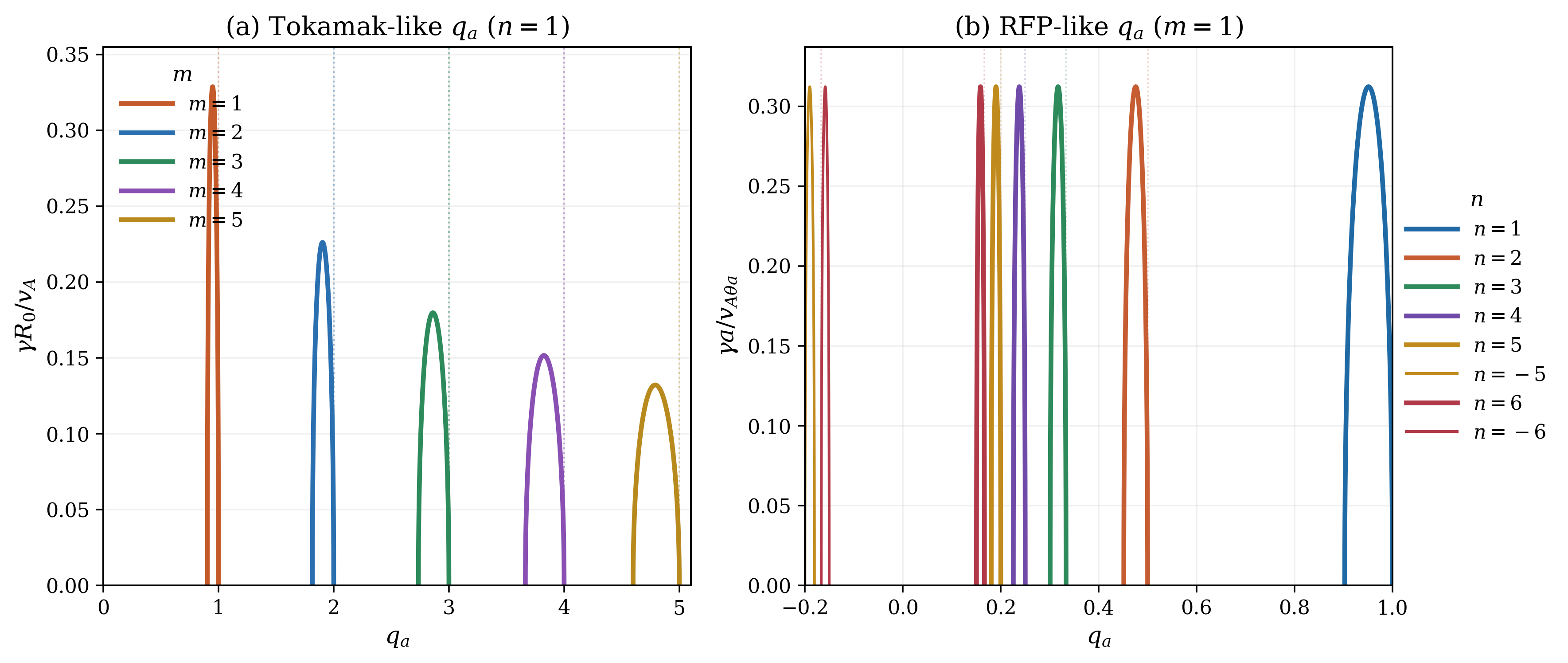
Writing \(v_A^2 = B_0^2/(\mu _0 \rho )\), this becomes

\boxed { \left (\frac {\gamma R_0}{v_A}\right )^2 = \frac {-4 (nq_a-m)\left [nq_a-(m-1+\alpha _m)\right ]} {q_a^2(1-\alpha _m)} } \qquad \left (\alpha _m=\left (\frac {a}{b}\right )^{2m}\right ).

Hence instability requires \(\gamma ^2>0\), i.e.

\frac {m-1+\alpha _m}{n} < q_a < \frac {m}{n}.

The resistive-wall continuation. Once the shell conductivity is finite, the ideal-wall increment \(\delta W_b^{\rm tok}\) is only partially restored. The thin-wall interpolation and dispersion relation derived in the Kruskal–Shafranov lecture, Eqs. (20.107) and (20.110), therefore give

\gamma \tau _w = -\frac {2b^2}{b^2-a^2} \frac {\delta W_\infty ^{\rm tok}}{\delta W_{\rm ideal}(b)}. \tag{22.42}

That is the slow RWM branch sitting just below the ideal-wall threshold. The same bookkeeping will reappear in Appendix E, where Eqs. (E.44) and (E.45) give the corresponding \(m=1\) RFP energies.

Constant-\(\lambda \) RFP analogue. The force-free Taylor equilibrium \(\curl \B =\lambda \B \) gives the RFP companion to the analytic constant-\(q\) exercise. Appendix E works the derivation through explicitly, starting from the Bessel core (E.26) and the edge safety-factor relation (E.32) and ending at Eqs. (E.37)–(E.42). In the same rigid-core \(m=1\) approximation used here, the result can be written as

\frac {\delta W_{m=1}^{\rm RFP}}{2\pi ^2 R_0/\muo } \simeq \frac {2B_{\theta a}^2}{1-\alpha _1} \,(nq_a-1)(nq_a-\alpha _1)\,|\xi _a|^2, \qquad \alpha _1=\left (\frac {a}{b}\right )^2, \tag{22.43}

with \(B_{\theta a}\equiv B_\theta (a)\). For a uniform-density rigid core,

\left (\frac {\gamma a}{v_{A\theta a}}\right )^2 \simeq \frac {-4 (nq_a-1)(nq_a-\alpha _1)}{1-\alpha _1}, \qquad v_{A\theta a}^2\equiv \frac {B_{\theta a}^2}{\mu _0\rho }. \tag{22.44}

So the same surface-energy logic predicts a low-\(q\) RFP band \(\alpha _1<nq_a<1\): the qualitative difference is that \(q_a<1\) lets several toroidal harmonics fit below the same upper root.

What these analytic profiles are good for. The constant-\(q\) profile is not the only choice. A constant-\(\lambda \) force-free profile leads to the familiar Bessel-function equilibrium, and its RFP free-boundary reduction is worked through in Appendix E, Eqs. (E.28)–(E.50). For the variational logic in the tokamak setting, the constant-\(q\) example is hard to beat because it makes the boundary ratio \(a\xi '/\xi \) analytic and therefore makes the stability bands, the no-wall/wall split, and the RWM continuation completely explicit.

22.4 From external kink to peeling modes

Why the edge problem is different. The external-kink calculation above treated the current profile as broad and the mode as a global boundary distortion. The edge of an H-mode tokamak is different. There the pressure pedestal produces a narrow region of strong parallel current density, usually a mixture of Ohmic, bootstrap, and Pfirsch–Schlüter current. A minimal sketch is

j_\parallel (r) = j_{\rm core}(r) + j_{\rm edge}\, \exp \!\left [-\frac {(a-r)^2}{\Delta _{\rm ped}^2}\right ], \qquad \Delta _{\rm ped}\ll a. \tag{22.45}

If the free energy is concentrated in this narrow outer layer, the minimizing ideal mode no longer looks like a broad external kink. It becomes radially localized at the edge and tries to peel the outer flux surfaces away from the core. That is why the tokamak edge literature calls it a peeling mode in the classic large-aspect-ratio edge literature of Connor et al. (1998); Wilson et al. (1999); Snyder et al. (2002).

What changes in the energy balance. In the cylindrical lecture the competition was between line bending, vacuum matching, and current drive at the moving edge. In the toroidal edge problem the bookkeeping becomes

\delta W_{\rm edge} \sim \delta W_{\rm bend} \;+\; \delta W_{\rm vac} \;+\; \delta W_{\rm Mercier} \;-\; \delta W_{j_\parallel (a)} . \tag{22.46}

The first two terms are the same stabilizing ingredients already familiar from the external kink. The last term is the destabilizing work done by the edge-localized parallel current. The new ingredient is \(\delta W_{\rm Mercier}\): once toroidal curvature and pressure-gradient effects are retained, the same Mercier/Suydam physics that later appears in the ballooning lecture contributes already here. In the large-aspect-ratio edge theory of Connor, Hastie, Wilson, and Miller, finite positive edge current is destabilizing, magnetic shear and vacuum energy are stabilizing, and the edge pressure gradient contributes a stabilizing Mercier-like term for the pure peeling branch Connor et al. (1998).

How the Newcomb analysis must be extended. The one-dimensional structure still begins from the ideal Euler–Lagrange equation

(f\xi ')'-g\xi =0, \tag{22.47}

but three extra pieces of physics must now be built into the coefficients and matching.

1.: The equilibrium profiles \(p(r)\), \(q(r)\), and \(j_\parallel (r)\) must be allowed to vary strongly across the pedestal, so the boundary ratio \(a\xi '(a)/\xi (a)\) is controlled by a thin edge layer rather than by a broad core solution.
2.: Toroidal curvature terms must be retained, because the pressure gradient no longer acts only as ballooning drive; it also enters the localized peeling criterion through a Mercier-like stabilizing contribution.
3.: A single cylindrical harmonic is no longer enough. Just as in the TAE chapter, toroidicity couples neighboring poloidal harmonics, so the edge problem is more naturally written as a banded system for \(\{\xi _{m-1},\xi _m,\xi _{m+1},\dots \}\), with the vacuum term still imposed at the plasma boundary.

Thus the real peeling problem is not a new instability in a new language. It is the external kink revisited for an edge-peaked current profile in toroidal geometry.

What is worth showing in these notes. For the purposes of these lecture notes, the important physics can be conveyed without reproducing the full pedestal formalism. One can show that replacing the broad constant-\(q\) profile by an edge current layer (22.45) pushes the minimizing external-kink eigenfunction toward the boundary and makes the mode radially localized. The result is an ideal current-driven external kink with finite displacement at the edge and strong sensitivity to \(j_\parallel (a)\), magnetic shear, and the vacuum region outside the plasma. That is the clean bridge to the modern pedestal picture.

Connection to peeling–ballooning and ELMs. At finite toroidal mode number the edge-current branch does not remain isolated. It couples to the pressure-driven ballooning branch, producing the peeling–ballooning modes that are widely used to interpret type-I ELM limits in H-mode pedestals Wilson et al. (1999); Snyder et al. (2002). The ballooning lecture should therefore be read as the pressure-gradient side of the same edge-stability story. There the emphasis shifts from \(j_\parallel (a)\) to curvature, magnetic shear, and field-line localization; here the key message is that a sufficiently large edge current can turn the external kink into an edge-localized, current-driven peeling mode.

Takeaways

This four-lecture sequence is the real payoff of Newcomb’s framework. We find:
1.
a one-dimensional variational formulation for the screw pinch;
2.
local pressure-driven tests (Suydam and Mercier);
3.
the fixed-boundary \(m=1\) internal kink when \(q_0<1\);
4.
external kink bands below each rational \(q_a=m/n\) once the wall solution is kept, together with the slow resistive-wall continuation when only a fraction of the ideal-wall increment survives;
5.
in toroidal edge geometry, the same current-driven external-kink physics reappears as an edge-localized peeling branch, which later couples to ballooning modes in the pedestal.

The wall does not merely shift a number. It changes the factorization of \(\delta W\) and introduces a second root. That is exactly why the diffuse-pinch problem is richer than the surface-current Kruskal–Shafranov model while still remaining close enough to it to teach from.

Bibliography

J. W. Connor, R. J. Hastie, H. R. Wilson, and R. L. Miller. Magnetohydrodynamic stability of tokamak edge plasmas. Physics of Plasmas, 5(7):2687–2700, 1998. doi:10.1063/1.872956.

H. R. Wilson, J. W. Connor, A. R. Field, S. J. Fielding, R. L. Miller, L. L. Lao, J. R. Ferron, and A. D. Turnbull. Ideal magnetohydrodynamic stability of the tokamak high-confinement-mode edge region. Physics of Plasmas, 6(5):1925–1932, 1999. doi:10.1063/1.873492.

P. B. Snyder, H. R. Wilson, J. R. Ferron, L. L. Lao, A. W. Leonard, T. H. Osborne, A. D. Turnbull, D. Mossessian, M. Murakami, and X. Q. Xu. Edge localized modes and the pedestal: A model based on coupled peeling–ballooning modes. Physics of Plasmas, 9(5):2037–2044, 2002. doi:10.1063/1.1449463.

Problems

Problem 22.1.: Starting from (21.93), rederive (21.99) and (21.100) without skipping the integration-by-parts step.
Problem 22.2.: Starting from (23.8), derive the Suydam criterion (23.17) and verify the factor of \(8\) in front of \(\muo p'/B_z^2\).
Problem 22.3.: Starting from (23.37), show that the toroidal correction relative to Suydam is \(\Delta _{\rm tor}=-q^2p'\). For \(p'<0\), determine the sign of the pressure term for \(q<1\), \(q=1\), and \(q>1\).
Problem 22.4.: For the analytic profile \(q(r)=q_a\), derive (22.27) explicitly for \(m=2\), \(n=1\) and identify the wall-stabilized interval in \(q_a\).
Problem 22.5.: Repeat the vacuum calculation leading to (22.11) for a no-wall plasma by taking \(b\rightarrow \infty \), and show directly that \(\Lambda _m\rightarrow 1\).