Lecture 23
Suydam and Mercier: Local Pressure-Driven Stability Tests
Overview
With Newcomb’s reduction in hand, the first internal danger is a localized
pressure-driven mode near a rational surface, where \(F(r_s)=0\) and field-line bending disappears.
Suydam gives the cylindrical criterion; Mercier gives the toroidal correction. These are
fixed-boundary tests: if they fail, the plasma is already unstable before any external-kink
calculation is relevant.
Historical Perspective
Newcomb’s 1960 paper is one of the classic stability papers in MHD because it
did not merely compute one growth rate or one threshold. It gave a framework.
The localized interchange limit near a rational surface is the part now associated
with Suydam’s criterion, while the toroidal generalization was clarified in the
work of Mercier and in the related local analyses of Greene, Johnson, and
Shafranov (Mercier, 1960) Mercier (1964) Greene and Johnson (1962) Shafranov and
Yurchenko (1968). The global boundary-value problem then became the natural
language for internal and external kink stability. Later cylindrical tokamak theory
is, in large part, Newcomb’s framework specialized to the large-aspect-ratio limit
Shafranov (1966); Freidberg (2014).
We now return to the reduced functional (21.92). Near a rational surface the coefficient \(f(r)\propto F^2\) becomes small, so
the dominant competition is between weakened line bending and pressure drive.
23.1 Suydam’s criterion
Focusing on internal modes we start with
\[\frac {\delta W}{2\pi ^2 R_0/\muo } = \int _0^{a} \left [ f(r)\,|\xi '|^2+g(r)\,|\xi |^2 \right ]dr\]
Localization near a rational surface.
Pressure-driven interchange-like perturbations localize near radii where field-line bending is weakest which
is where
\[f = \frac {rF^2}{k_0^2}\]
and \[F = \frac {m B_\theta }{r} + k B_z = \frac {B_z}{R_0}\left (\frac {m}{q(r)}-n\right )\]
\[k_0^2 = \frac {m^2}{a^2} + \frac {n^2}{R_0^2}\]
\[F(r_s)=\B \cdot \bm {k}=0 \qquad \Longleftrightarrow \qquad q(r_s)=\frac {m}{n} \tag{23.5}\]
recalling that the field line bending energy is \(\delta W_{bend} \propto B^2 k_\parallel ^2 \xi ^2\) and so the rational surface is where \(k_\parallel = 0\) for the
large-aspect-ratio sign convention \(k=-n/R_0\) used later. Expand \[F(r)\simeq F'(r_s)\,x, \qquad x\equiv r-r_s, \tag{23.6}\]
and assume \(\xi \) is sharply localized in \(x\). Examing \[g(r) = \underbrace {\frac {2k^2}{k_0^2}\,\muo p'}_{\text {pressure drive}} + \left (\frac {k_0^2r^2-1}{k_0^2r^2}\right )\cancelto {0}{rF^2} + \frac {2k^2}{r k_0^4} \left (kB_z-\frac {mB_\theta }{r}\right )\cancelto {0}{F}. \tag{23.7}\]
.
Then (21.92) reduces to
\[\frac {\delta W}{2\pi ^2 R_0/\muo } \simeq \frac {r_s[F'(r_s)]^2}{k^2+m^2/r_s^2} \int _{-\infty }^{\infty } \left [ x^2\left (\pp {\xi }{x}\right )^2 - D_s\,\xi ^2 \right ]dx, \tag{23.8}\]
with \[D_s \equiv -\frac {2\muo k^2}{r_s[F'(r_s)]^2}\,p'(r_s). \tag{23.9}\]
Connection to magnetic shear.
In the large-aspect-ratio ordering,
\[q(r)=\frac {rB_z}{R_0 B_\theta }, \qquad k=-\frac {n}{R_0},\]
and at resonance \(q(r_s)=m/n\). One finds \[F'(r_s) = -\frac {mB_z(r_s)}{R_0q^2(r_s)}\,q'(r_s) = -\frac {nB_z(r_s)}{R_0q(r_s)}\,q'(r_s). \tag{23.11}\]
Therefore \[D_s = -\frac {2\muo q^2(r_s)}{r_s B_z^2(r_s)\,[q'(r_s)]^2}\,p'(r_s). \tag{23.12}\]
Euler–Lagrange equation and the threshold.
Varying (23.8) gives
\[\dd {}{x}\left (x^2\dd {\xi }{x}\right )+D_s\,\xi =0. \tag{23.13}\]
Try a power law \(\xi \sim x^p\). Then \[p(p+1)+D_s=0, \qquad p=\frac {-1\pm \sqrt {1-4D_s}}{2}. \tag{23.14}\]
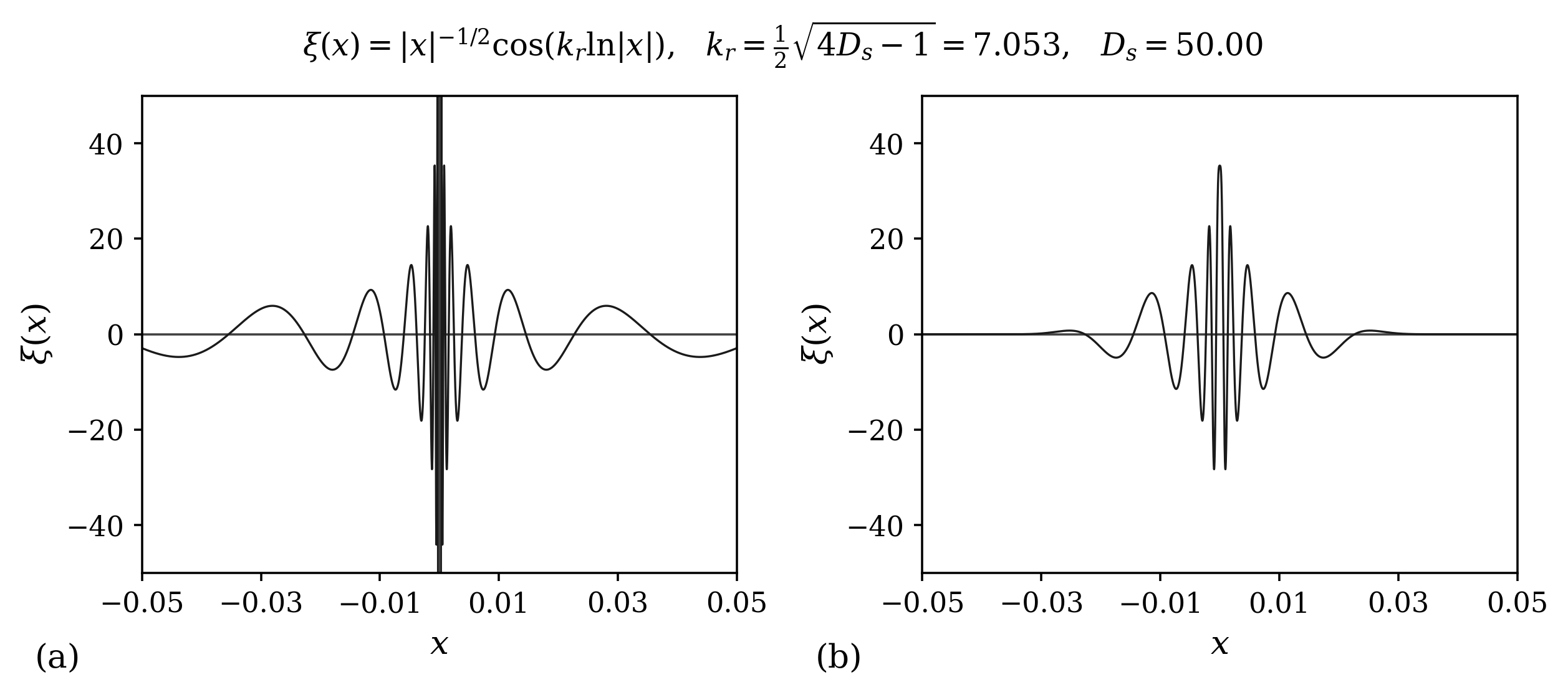
If \(D_s>1/4\), the exponent is complex and the solution becomes log-oscillatory, \[\xi (x) = \frac {1}{|x|^{1/2}} \left [ c_1\sin \!\left (k_r\ln |x|\right ) + c_2\cos \!\left (k_r\ln |x|\right ) \right ], \qquad k_r=\frac {1}{2}\sqrt {4D_s-1}, \tag{23.15}\]
which signals interchange-like instabilityas shown in Fig. 23.1. Thus \[D_s\le \frac {1}{4} \tag{23.16}\]
is the local stability condition. Using (23.12), this becomes the usual Suydam form \[\frac {r_s B_z^2(r_s)}{8\muo } \left (\frac {q'(r_s)}{q(r_s)}\right )^2 + p'(r_s) \ge 0, \tag{23.17}\]
or equivalently \[\left (\frac {r_s q'(r_s)}{q(r_s)}\right )^2 + \frac {8\muo r_s p'(r_s)}{B_z^2(r_s)} \ge 0.\]
Since \(p'<0\) in the usual case, magnetic shear stabilizes by making the first term large.
23.2 Mercier’s toroidal correction
Start from the same toroidal energy principle as ballooning.
The cleanest way to introduce Mercier is not to start from a different theory, but from the same
axisymmetric tokamak energy functional used in Lecture 26. Equation (26.6) there is the exact
two-dimensional ideal-MHD volume contribution in flux coordinates, and Appendix I shows in detail how
to eliminate \(\xi _\parallel \) and then reduce the problem to an \(X\)-only functional. For the present lecture we do not need to
repeat that algebra. We simply borrow the result and specialize it to the local pressure-driven
channel.
Concretely, we suppress the localized current-driven contribution by setting \(J_\parallel =0\) in the Mercier discussion.
More precisely, in the appendix functional (I.76) this means dropping the \(\sigma ' \sim dJ_\parallel /d\Psi \) terms, so that only
pressure-gradient and curvature drive remain. In the localized-mode ordering this gives the toroidal
analogue of the Suydam functional,
\[\begin {aligned} \delta W = \pi \int J\,d\Psi \,d\chi \Biggl [ &\frac {B^2}{R^2B_p^2}\,|k_\parallel X|^2 + R^2B_p^2 \left | \frac {1}{n}\frac {\partial }{\partial \Psi }(k_\parallel X) \right |^2 \\[0.4em] &\qquad - 2p' \left ( \frac {\kappa _n}{RB_p}|X|^2 - i\,\frac {\muo I_{\mathrm {pol}}\kappa _g}{B^2}\, X\,\frac {\partial X^*}{n\,\partial \Psi } \right ) \Biggr ], \end {aligned} \tag{23.19}\]
which is the form emphasized in Zohm’s notes. The new ingredients relative to the cylinder are the
curvature components \[\begin{aligned}\kappa _n &= \frac {RB_p}{B^2}\frac {\partial }{\partial \Psi } \left (\muo p+\frac {B^2}{2}\right ), \\ \kappa _g &= -\frac {1}{JB_pB^2}\frac {\partial }{\partial \chi }\left (\frac {B^2}{2}\right ),\end{aligned} \tag{23.20}\]
namely the normal curvature and the geodesic curvature.
Historical Perspective
Mercier as the toroidal completion of Suydam. The point of (23.19) is structural.
In a cylinder, the pressure term is just a local number multiplying \(|X|^2\). In a torus, that same
pressure gradient couples to curvature, and curvature varies around the flux surface. So
the local criterion can no longer depend only on shear and \(p'\); it must also know how a field
line samples good and bad curvature as it winds around the torus. That is the physical
content of Mercier’s generalization.
Localized interchange ansatz.
To isolate interchange-like modes, choose the phase so that it is constant along the equilibrium field line on
the resonant surface \(\Psi =\Psi _0\):
\[X(\Psi ,\chi ,\phi ) = \widehat X(\Psi ,\chi ) \exp \!\left \{ in\left [ \phi -\int _0^\chi \nu (\Psi _0,\chi ')\,d\chi ' \right ] \right \}. \tag{23.22}\]
This is the toroidal replacement for fixing a single helical phase in the screw pinch. The important
difference is that the poloidal harmonic number is no longer a good quantum number by itself. Instead, the
phase must follow the field-line pitch \(\nu (\Psi ,\chi )\).
Now localize sharply around the resonant surface by introducing
\[x \equiv n^2(\Psi -\Psi _0), \qquad \widehat X(\Psi ,\chi ) = X_0(x)+\frac {1}{n}X_1(x,\chi )+\cdots . \tag{23.23}\]
The dominant piece \(X_0\) is a slowly varying envelope in the stretched radial coordinate, while \(X_1\) carries the
poloidal sideband correction forced by toroidicity. Minimizing with respect to \(X_1\) produces a functional of
exactly the same singular form as in the screw pinch, \[\delta W = C_M \int _{-\infty }^{\infty } dx\, \left [ x^2\left (\frac {dX_0}{dx}\right )^2 - D_M\,X_0^2 \right ], \tag{23.24}\]
where the prefactor \[C_M = \frac {\pi ^3}{n^2} \left (\frac {dq}{d\Psi _0}\right )^2 \left ( \oint \frac {\nu B^2}{B_p^2}\,d\chi \right )^{-1} \muo I_{\mathrm {pol}} \tag{23.25}\]
is positive and therefore does not affect the sign of \(\delta W\). All of the stability information sits in the toroidal
index \(D_M\).
The Euler–Lagrange equation and the new effective potential.
Varying (23.24) gives
\[\frac {d}{dx}\left ( x^2\frac {dX_0}{dx} \right ) + D_M\,X_0 = 0. \tag{23.26}\]
It is convenient to rewrite this in exactly the same notation as the singular local equation we used before:
\[\hat U_M \equiv -D_M , \tag{23.27}\]
so that \[\frac {d}{dx}\left ( x^2\frac {dX_0}{dx} \right ) - \hat U_M\,X_0 = 0. \tag{23.28}\]
This is the precise sense in which “our \(U_m\) now has extra terms.” The operator is the same singular
Newcomb/Suydam operator, but the effective potential has been renormalized by toroidicity:
\[\hat U_M = \underbrace {\hat U_S}_{\text {cylindrical pressure/shear}} + \underbrace {\Delta \hat U_{\kappa _n}}_{\text {normal curvature}} + \underbrace {\Delta \hat U_{\rm PS}}_{\text {geodesic/Pfirsch--Schl{\"u}ter}}. \tag{23.29}\]
The cylinder had only the first piece. Mercier keeps the other two.
A geometric form of the Mercier index, following Zohm, is
\[D_M = \frac {\muo \,dp/d\Psi _0}{(dq/d\Psi _0)^2} \left \langle \frac {R^2B_p^2}{JB^2} \right \rangle ^{-2} \left [ 2\left \langle \frac {RB_p\kappa _n}{B^2}\right \rangle + \left \langle \frac {\Lambda _M}{B^4}\right \rangle - \left \langle \frac {1}{B^2}\right \rangle \left \langle \frac {\Lambda _M}{B^2}\right \rangle \right ], \tag{23.30}\]
with the surface average \[\langle f\rangle \equiv \left ( \oint \frac {B^2}{R^2B_p^2}J\,d\chi \right )^{-1} \oint \frac {f B^2}{R^2B_p^2}J\,d\chi . \tag{23.31}\]
Here \(\Lambda _M\) is the standard Pfirsch–Schlüter/shear combination on the resonant surface. The crucial point is not
the bookkeeping of \(\Lambda _M\), but the physics encoded by (23.30): Mercier is driven by the pressure
gradient times curvature. The first extra term is the surface-averaged normal curvature, while
the remaining terms come from the parallel force balance that sets up the Pfirsch–Schlüter
response.
The criterion itself.
Because (23.28) has the same singular structure as the Suydam equation, the same indicial analysis
applies. Trying
\[X_0\sim |x|^p\]
gives \[p(p+1)+D_M=0. \tag{23.33}\]
Once again the transition from monotonic to log-oscillatory behavior occurs at \[D_M=\frac {1}{4}.\]
So the local ideal-MHD Mercier criterion is \[D_M\le \frac {1}{4}. \tag{23.35}\]
Mathematically, this is the same threshold as Suydam. Physically, the difference is that \(D_M\) now contains
toroidal curvature and Pfirsch–Schlüter structure.
Reduction to the cylinder and to the circular tokamak.
The geometric formula (23.30) makes the cylindrical limit easy to read. For a screw pinch with \(R=R_0\),
\(B_p=B_\theta (r)\), and \(B\simeq B_z\), the Pfirsch–Schlüter/geodesic terms cancel, so one recovers the cylindrical Suydam
index. In other words, Mercier really is the toroidal completion of Suydam, not a different local
instability.
For a torus with cylindrical flux surfaces the criterion reduces to the familiar large-aspect-ratio form.
Instability occurs when
\[-\frac {8\muo p'}{r_{\rm res}B_z^2} \left (1-q^2\right ) > \left (\frac {q'}{q}\right )^2, \tag{23.36}\]
or, equivalently, stability requires \[\frac {r_{\rm res}B_z^2}{8\muo } \left (\frac {q'}{q}\right )^2 + p'(r_{\rm res})\left (1-q^2(r_{\rm res})\right ) \ge 0 . \tag{23.37}\]
So the cylindrical Suydam balance \[\underbrace { \frac {r_s B_z^2}{8\muo }\left (\frac {q'}{q}\right )^2+p' }_{\text {Suydam}} \qquad \longrightarrow \qquad \underbrace { \frac {r_s B_z^2}{8\muo }\left (\frac {q'}{q}\right )^2 + p'\left (1-q^2\right ) }_{\text {Mercier}} \tag{23.38}\]
acquires an explicitly toroidal correction. For the usual case \(p'<0\), the factor \((1-q^2)\) shows immediately why
toroidicity can stabilize localized interchange once \(q>1\).
Caution
Mercier is not yet ballooning. In Mercier theory the phase is chosen to be constant along
the resonant field line, and the curvature drive is then averaged over the whole flux
surface. The ballooning lecture relaxes that restriction and lets the mode choose where
along the field line it wants to live. That is why the same pressure–curvature physics
that looks surface-averaged in (23.19) reappears as a strongly localized bad-curvature
drive in the ballooning equations (26.70), (26.68), and in the appendix bridge equation
(I.136).
Takeaways
There are really three local pressure-driven lectures hiding inside one story.
Suydam is the cylindrical rational-surface test: can magnetic shear beat the local pressure
drive?
Mercier is the axisymmetric toroidal ideal-MHD refinement: the same singular
equation reappears, but now the effective potential picks up normal-curvature and
Pfirsch–Schlüter terms, so pressure drive must be judged together with how the field
line samples curvature around the torus.
Ballooning comes next: instead of averaging the curvature over the surface, we let the
perturbation localize in the bad-curvature region, which leads to the field-line problem of
Lecture 26. And in the resistive interchange lecture, the same pressure–curvature drive
returns once more, but with finite resistivity relaxing the ideal frozen-in constraint at
the rational surface. So Mercier is the right bridge lecture: it is where curvature first
enters the local ideal-MHD criterion in a systematic toroidal way.
Bibliography
Claude Mercier. A necessary condition for hydromagnetic stability of plasma with axial symmetry. Nuclear Fusion, 1(1):47–53, 1960. doi:10.1088/0029-5515/1/1/004.
Claude Mercier. Equilibrium and stability of a toroidal magnetohydrodynamic system in the neighbourhood of a magnetic axis. Nuclear Fusion, 4(3):213–226, 1964. doi:10.1088/0029-5515/4/3/008.
John M. Greene and John L. Johnson. Stability criterion for arbitrary hydromagnetic equilibria. Physics of Fluids, 5(5):510–517, 1962.
V. D. Shafranov and E. I. Yurchenko. Condition for flute instability of a toroidal-geometry plasma. Soviet Physics JETP, 26:682–686, 1968.
V. D. Shafranov. Plasma equilibrium in a magnetic field. In M. A. Leontovich, editor, Reviews of Plasma Physics, volume 2, pages 103–151. Consultants Bureau, New York, 1966. Classic long review; includes the large-aspect-ratio treatment used for what is commonly called the Shafranov shift.
Jeffrey P. Freidberg. Ideal MHD. Cambridge University Press, Cambridge, UK, 2014. ISBN 9781107006256. Fully updated successor to *Ideal Magnetohydrodynamics*.