Kinetic MHD: Collisionless Pressure Response

← Previous Lecture Contents Next Lecture →

Lecture 15
Kinetic MHD: Collisionless Pressure Response

Overview

Kinetic MHD keeps the low-frequency MHD force law but replaces the pressure closure.
1.
The magnetic geometry, field-line bending, and frozen-in motion are still governed by the same low-frequency framework developed in the flux-freezing lecture, in Lecture 4, and in Lecture 14.
2.
The new physics enters through the collisionless pressure response, obtained from the drift-kinetic equation rather than from a fluid closure.
3.
The main lesson is beautifully sharp: the firehose mode is already visible in anisotropic fluid theory, while the mirror mode is the place where the kinetic closure changes the quantitative answer.
4.
A useful bonus is that restoring the appropriate pieces of generalized Ohm’s law shows how two-fluid and kinetic effects begin to feed into inertial Alfvén waves, kinetic Alfvén waves, and eventually Hall and FLR corrections.

Historical Perspective

The CGL closure showed in 1956 that a magnetized collisionless plasma can still be described by a fluid system, provided one respects the magnetic-field direction and the adiabatic invariants Chew et al. (1956). The next step was to recognize that not every low-frequency problem is captured accurately by a local fluid closure. Kulsrud’s treatment made the low-frequency bridge from MHD to drift-kinetic theory especially clear Kulsrud (1983). For anisotropy-driven instabilities, the classic mirror calculations of Vedenov and Sagdeev and the later drift-mirror analysis of Hasegawa showed explicitly where the kinetic response changes the answer Vedenov and Sagdeev (1958a,b); Hasegawa (1969). The physical mechanism of the mirror mode was later clarified in a particularly transparent way by Southwood and Kivelson Southwood and Kivelson (1993). The modern language “kinetic MHD” is therefore well chosen: it is still MHD in its force balance, but kinetic in its closure.

Kinetic MHD sits in the gap between ideal fluid theory and full kinetic theory. It is still a long-wavelength, low-frequency theory, so the magnetic field and bulk motion are treated in an MHD spirit. But it refuses to guess the pressure response. Instead it computes that response from the kinetic equation. That is why this lecture is worth separating from the ordinary Alfvén-wave lecture: it is not merely another dispersion relation, but a different lesson about how plasma theory is organized.

15.1 What kinetic MHD keeps and what it changes

Ordering. We retain the low-frequency, magnetized ordering

\omega \ll \Omega _i, \qquad k_\perp \rho _i \ll 1, \tag{15.1}

so the frozen-in relation of Eq. (2.13) and the basic low-frequency force balance of Eq. (1.8) remain useful. What is not assumed is rapid collisional relaxation to a local Maxwellian.

Force law versus closure. The cleanest bridge from Chapter 11 is simply to restore the inertial terms in the gyrotropic force balance. For a low-frequency plasma with \(\vect {u}=u_\parallel \vect {b}+\delta \vect {u}\), the time-dependent parallel and perpendicular balances may be written schematically as

\begin{aligned}\rho \frac {d u_\parallel }{dt} &= - \left [ \pp {p_\parallel }{\ell } + \frac {p_\perp -p_\parallel }{B}\pp {B}{\ell } \right ], \\ \rho \frac {d \vect {u}_\perp }{dt} &= - \grad _\perp \left (p_\perp +\frac {B^2}{2\muo }\right ) + \left (\frac {B^2}{\muo }+p_\perp -p_\parallel \right )\vect {\kappa }.\end{aligned} \tag{15.2}

These are just the Chapter 11 force-balance equations with inertia restored. Kinetic MHD keeps this MHD-looking force law and changes only the closure that determines \(\delta p_\perp \) and \(\delta p_\parallel \).

In a uniform anisotropic equilibrium with \(\B _0=B_0\vect {e}_z\) and \(\vect {k}=k_\perp \vect {e}_x+k_\parallel \vect {e}_z\), the linearized momentum equation still has the same geometric pieces as in the previous lecture. For the compressive branch follows directly from perpendicular and parallel force balance: one may write schematically

\begin{aligned}-\omega ^2 \rho _0 \vect {\xi }_\perp &= - i\vect {k}_\perp \left ( \delta p_\perp + \frac {B_0\delta B}{\muo } \right ) - k_\parallel ^2 \left ( \frac {B_0^2}{\muo }+p_{\perp 0}-p_{\parallel 0} \right )\vect {\xi }_\perp , \\ -\omega ^2 \rho _0 \xi _\parallel &= - i k_\parallel \left [ \delta p_\parallel + \left (p_{\perp 0}-p_{\parallel 0}\right )\frac {\delta B}{B_0} \right ].\end{aligned} \tag{15.4}

These are still MHD-looking equations. The real question is: what are \(\delta p_\perp \) and \(\delta p_\parallel \)? In CGL they come from the double-adiabatic laws. In kinetic MHD they come from the drift-kinetic equation.

The lesson in one sentence. If a mode mainly tests magnetic tension, CGL and kinetic MHD often agree. If a mode mainly tests compressive pressure balance, the kinetic closure matters. That is why the firehose threshold is already visible in Eq. (14.46), while the mirror threshold needs to be re-derived.

15.2 Drift-kinetic pressure response of a bi-Maxwellian plasma

Geometry and variables. Take a uniform equilibrium field

\B _0 = B_0 \vect {e}_z, \qquad \delta B \equiv \delta B_\parallel , \qquad E_\parallel = - i k_\parallel \tilde {\Phi }, \qquad \propto e^{-i\omega t + i k_\parallel z}. \tag{15.6}

For compressive perturbations,

\frac {\delta B}{B_0} = - i \vect {k}_\perp \cdot \vect {\xi }_\perp . \tag{15.7}

Use guiding-center variables \((\mu ,v_\parallel )\), where

\mu \equiv \frac {m_s v_\perp ^2}{2B_0}. \tag{15.8}

The equilibrium distribution for each species is taken to be bi-Maxwellian:

f_{0s}(\mu ,v_\parallel ) = n_0 \frac {m_s}{2\pi T_{\perp s}} \left (\frac {m_s}{2\pi T_{\parallel s}}\right )^{1/2} \exp \left ( -\frac {m_s v_\parallel ^2}{2T_{\parallel s}} -\frac {\mu B_0}{T_{\perp s}} \right ). \tag{15.9}

It is convenient to define

A_s \equiv \frac {T_{\perp s}}{T_{\parallel s}}, \qquad v_{{\rm th}\parallel s} \equiv \sqrt {\frac {2T_{\parallel s}}{m_s}}, \qquad x_s \equiv \frac {v_\parallel }{v_{{\rm th}\parallel s}}, \qquad \zeta _s \equiv \frac {\omega }{k_\parallel v_{{\rm th}\parallel s}}. \tag{15.10}

Linearized drift-kinetic equation. The parallel part of the drift-kinetic equation is

-i(\omega -k_\parallel v_\parallel ) f_{1s} + \left ( \frac {q_s}{m_s}E_\parallel - \frac {\mu }{m_s} i k_\parallel \delta B \right ) \pp {f_{0s}}{v_\parallel } =0. \tag{15.11}

For the bi-Maxwellian equilibrium,

\pp {f_{0s}}{v_\parallel } = -\frac {m_s v_\parallel }{T_{\parallel s}} f_{0s}. \tag{15.12}

Insert \(E_\parallel =-ik_\parallel \tilde {\Phi }\) and Eq. (15.12) into Eq. (15.11):

\begin{aligned}f_{1s} &= \frac {k_\parallel v_\parallel }{\omega -k_\parallel v_\parallel } \left ( \frac {q_s\tilde {\Phi }}{T_{\parallel s}} + \frac {\mu \delta B}{T_{\parallel s}} \right )f_{0s} \nonumber \\ &= \frac {x_s}{\zeta _s-x_s} \left ( \frac {q_s\tilde {\Phi }}{T_{\parallel s}} + \frac {\mu B_0}{T_{\parallel s}}\frac {\delta B}{B_0} \right )f_{0s}.\end{aligned} \tag{15.13}

This formula already shows the central resonance: \(\omega -k_\parallel v_\parallel \).

Plasma-dispersion notation. Introduce

Z(\zeta ) = \frac {1}{\sqrt {\pi }} \int _{-\infty }^{\infty } \frac {e^{-x^2}}{x-\zeta }\,dx, \qquad R(\zeta )\equiv 1+\zeta Z(\zeta ), \tag{15.14}

and define \(R_s\equiv R(\zeta _s)\). The required Gaussian integrals are

\frac {1}{\sqrt {\pi }} \int _{-\infty }^{\infty } \frac {x e^{-x^2}}{\zeta -x}\,dx = - R(\zeta ), \tag{15.15}

and

\frac {1}{\sqrt {\pi }} \int _{-\infty }^{\infty } \frac {x^3 e^{-x^2}}{\zeta -x}\,dx = -\left (\frac {1}{2}+\zeta ^2 R(\zeta )\right ). \tag{15.16}

Density and pressure moments. At fixed \((\mu ,v_\parallel )\), the phase-space measure is

d^3v = \frac {2\pi B_0}{m_s}\,d\mu \,dv_\parallel . \tag{15.17}

Evaluating the moments gives

\begin{aligned}\frac {\delta n_s}{n_0} &= \left [1-A_s R_s\right ]\frac {\delta B}{B_0} - R_s\frac {q_s\tilde {\Phi }}{T_{\parallel s}}, \\[4pt] \delta p_{\perp s} &= 2p_{\perp s}\left [1-A_s R_s\right ]\frac {\delta B}{B_0} - p_{\perp s} R_s \frac {q_s\tilde {\Phi }}{T_{\parallel s}}, \\[4pt] \delta p_{\parallel s} &= p_{\parallel s} \left [1-A_s\left (1+2\zeta _s^2R_s\right )\right ]\frac {\delta B}{B_0} - p_{\parallel s}\left (1+2\zeta _s^2R_s\right )\frac {q_s\tilde {\Phi }}{T_{\parallel s}}.\end{aligned} \tag{15.18}

For singly charged ions and electrons, quasineutrality \(\delta n_i=\delta n_e\) gives

\boxed { e\tilde {\Phi } = \frac {A_eR_e-A_iR_i} {R_i/T_{\parallel i}+R_e/T_{\parallel e}} \frac {\delta B}{B_0}. } \tag{15.21}

Equations (15.18)–(15.21) are the core of kinetic MHD for this problem.

15.3 Slow mirror ordering

Low-frequency limit. The mirror and long-wavelength firehose instabilities live in the regime

|\zeta _s| = \left |\frac {\omega }{k_\parallel v_{{\rm th}\parallel s}}\right |\ll 1, \qquad \Longrightarrow \qquad R_s \to 1. \tag{15.22}

Then Eq. (15.21) becomes

e\tilde {\Phi } = \frac {A_e-A_i} {1/T_{\parallel i}+1/T_{\parallel e}} \frac {\delta B}{B_0}. \tag{15.23}

Equal anisotropy or vanishing \(E_\parallel \). A particularly clean limit is

A_i=A_e\equiv A, \qquad \tilde {\Phi }=0. \tag{15.24}

Then Eqs. (15.18)–(15.20) reduce to

\begin{aligned}\frac {\delta n}{n_0} &= (1-A)\frac {\delta B}{B_0}, \\ \delta p_{\parallel s} &= p_{\parallel s}(1-A)\frac {\delta B}{B_0}, \\ \delta p_{\perp s} &= 2p_{\perp s}(1-A)\frac {\delta B}{B_0}.\end{aligned} \tag{15.25}

These are the formulas used below to derive the simplest collisionless mirror threshold.

15.4 Firehose: loss of field-line tension

Transverse polarization. Take a purely shear perturbation

\vect {\xi } = \xi _y \vect {e}_y, \qquad \vect {k}\cdot \vect {\xi }=0, \qquad \frac {\delta B}{B_0}=0. \tag{15.28}

Then the kinetic pressure response drops out because the perturbation is incompressible and contains no \(\delta B_\parallel \). The perturbed magnetic field is

\B _1 = i k_\parallel B_0 \xi _y \vect {e}_y, \tag{15.29}

so the field-direction perturbation is

\vect {b}_1 = i k_\parallel \xi _y \vect {e}_y. \tag{15.30}

Force balance. The magnetic tension force is

\frac {1}{\muo }(i\vect {k}\times \B _1)\times \B _0 = - \frac {B_0^2}{\muo }k_\parallel ^2 \xi _y \vect {e}_y. \tag{15.31}

The anisotropic pressure tensor contributes

-\left (\divergence \tens {P}_1\right )_y = -\left (p_{\perp 0}-p_{\parallel 0}\right )k_\parallel ^2\xi _y. \tag{15.32}

Hence

-\omega ^2 \rho _0 \xi _y = - k_\parallel ^2 \left ( \frac {B_0^2}{\muo }+p_{\perp 0}-p_{\parallel 0} \right )\xi _y. \tag{15.33}

Therefore

\boxed { \omega ^2 = k_\parallel ^2 \frac {B_0^2/\muo +p_{\perp 0}-p_{\parallel 0}}{\rho _0}. } \tag{15.34}

This is exactly the same result as Eq. (14.45). The firehose threshold is therefore

\boxed { p_{\parallel 0}-p_{\perp 0} > \frac {B_0^2}{\muo }. } \tag{15.35}

The lesson. The firehose mode is already present in anisotropic fluid theory because its physics is the sign of the field-line tension. The closure hardly enters. In that sense the firehose instability is the easiest anisotropy-driven mode to understand.

15.5 Mirror: failure of compressive balance

Oblique compressive perturbation. Now take a compressive perturbation in the \(x\)–\(z\) plane. From Eq. (15.7),

\frac {\delta B}{B_0} = - i k_\perp \xi _x, \qquad \frac {\delta \B _\perp }{B_0} = i k_\parallel \vect {\xi }_\perp . \tag{15.36}

The perturbed curvature of an initially straight field line is

\vect {\kappa }_1 = (\vect {b}\cdot \grad )\vect {b}_1 = i k_\parallel \vect {b}_1 = - k_\parallel ^2 \vect {\xi }_\perp . \tag{15.37}

Take the divergence of the perpendicular force balance (15.4) and use Eq. (15.7). One obtains

\boxed { \omega ^2 \frac {\delta B}{B_0} = k_\perp ^2 \left ( \frac {\delta p_\perp }{\rho _0} + v_A^2 \frac {\delta B}{B_0} \right ) + k_\parallel ^2 \left ( v_A^2 + c_\perp ^2 - c_\parallel ^2 \right ) \frac {\delta B}{B_0}. } \tag{15.38}

The parallel force balance is

-\omega ^2 \rho _0 \xi _\parallel = - i k_\parallel \left [ \delta p_\parallel + \left (p_{\perp 0}-p_{\parallel 0}\right )\frac {\delta B}{B_0} \right ]. \tag{15.39}

In the slow limit this says that the parallel force is nearly balanced, so the mirror mode is oblique rather than exactly perpendicular.

Insert the kinetic closure. Use the slow-ordering response (15.27):

\delta p_\perp = 2p_{\perp 0}(1-A)\frac {\delta B}{B_0}, \qquad A \equiv \frac {T_\perp }{T_\parallel }. \tag{15.40}

Equation (15.38) becomes

\begin{aligned}\omega ^2 &= k_\perp ^2 \left [ v_A^2 + 2\frac {p_{\perp 0}}{\rho _0}(1-A) \right ] + k_\parallel ^2 \left ( v_A^2+c_\perp ^2-c_\parallel ^2 \right ) \nonumber \\ &= k_\perp ^2 v_A^2 \left [ 1+\beta _\perp ^\ast (1-A) \right ] + k_\parallel ^2 \left ( v_A^2+c_\perp ^2-c_\parallel ^2 \right ),\end{aligned} \tag{15.41}

where for compactness we defined

\beta _\perp ^\ast \equiv \frac {2p_{\perp 0}}{\rho _0 v_A^2} = \frac {2\muo p_{\perp 0}}{B_0^2}. \tag{15.42}

The mirror mode is most unstable for \(k_\perp \gg k_\parallel \), so the first term controls the threshold:

1+\beta _\perp ^\ast (1-A) < 0. \tag{15.43}

Thus the simplest kinetic-MHD mirror criterion is

\boxed { \frac {T_\perp }{T_\parallel } > 1+\frac {1}{\beta _\perp ^\ast }. } \tag{15.44}

It is also interesting that this "magnetosonic" branch also has a second type of firehose instability. It, like the mirror is oblique but becomes large when the parallel wavelength is short and \(k_\parallel \gg k_\perp \). The firehose condition governing stability is exactly the same as before but the character of the wave is no longer a shear but rather compressional.

Comparison with CGL. Compare Eq. (15.44) with the CGL result (14.54). The magnetic part of the force balance is the same in both cases. The difference is entirely in the compressive pressure response. That is why it is worth separating this lecture from the ordinary wave lecture: the mirror mode is the cleanest example of a low-frequency problem whose geometry is fluid-like but whose closure is kinetic.

A useful physical picture. The mirror mode bunches magnetic flux so that some regions have larger \(B\) and some smaller \(B\). When \(T_\perp >T_\parallel \), particles with large magnetic moment prefer the weaker-\(B\) regions. That pile-up raises the perpendicular pressure where the field is already weak, which further deepens the magnetic well. The mode is therefore a compressive anti-restoring response. Southwood and Kivelson’s discussion makes this picture especially transparent Southwood and Kivelson (1993).

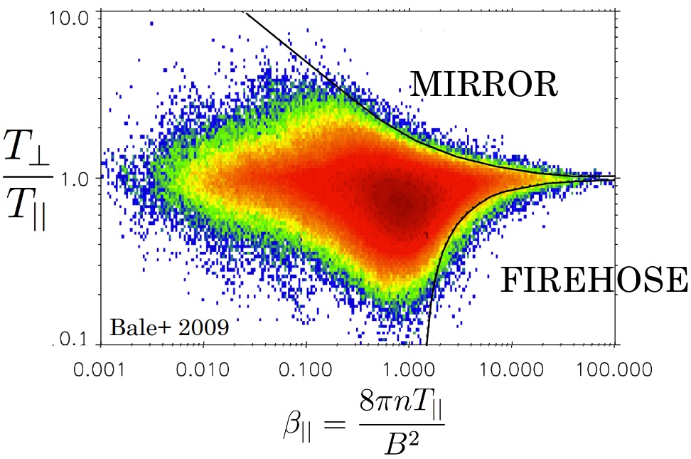
Figure 15.1: Solar-wind proton anisotropy data with mirror and firehose thresholds overlaid. The point of the figure is not merely observational: nature actually populates the kinetic-MHD marginality boundaries. Bale et al. (2009)

Observational perspective. The expanding solar wind provides the cleanest natural laboratory for these anisotropy-driven instabilities. As the plasma expands, \(T_\perp /T_\parallel \) is driven away from unity, but the proton distribution is observed to remain bounded by the mirror and oblique-firehose thresholds rather than wandering freely in anisotropy space Hellinger et al. (2006); Bale et al. (2009). That is a beautiful confirmation of the kinetic-MHD point of view: the plasma evolves under low-frequency MHD-like dynamics, but kinetic microinstabilities regulate the pressure tensor.

15.6 Adding back two-fluid effects: inertial and kinetic Alfvén waves

Why this comes after the mirror and firehose discussion. Up to this point the lecture has stayed within strict kinetic MHD: the low-frequency MHD force law is kept, but the pressure closure is replaced by the drift-kinetic response. The next step is a genuine change in approach. One now begins to add back the two-fluid corrections that were dropped on the way from the generalized Ohm law (3.10) to ideal MHD. That is where inertial Alfvén waves, kinetic Alfvén waves, and eventually finite- Larmor-radius corrections begin to appear.

What has to be added. The force balance of Lecture 17 already contains the correct Alfvénic geometry: field-line bending supplies the restoring force, while compressibility enters through \(\delta n\), \(\delta p\), and \(E_\parallel \). What strict kinetic MHD suppressed was the part of generalized Ohm’s law that allows a small but finite parallel electric field. In the notation written in Eq. (3.10), the relevant straight-field, collisionless, isotropic limit is

E_\parallel = - \frac {T_e}{e}\vect {b}\cdot \grad \left (\frac {\delta n}{n_0}\right ) - \frac {m_e}{n_0 e^2}\pp {J_\parallel }{t}. \tag{15.45}

The first term is the adiabatic or Boltzmann electron response along the field line; the second is electron inertia. Those are precisely the terms that generate kinetic and inertial Alfvén waves Hasegawa and Chen (1975, 1976); Goertz and Boswell (1979); Lysak and Lotko (1996).

Shear geometry with finite \(E_\parallel \). Take an isotropic equilibrium with

\B _0 = B_0 \vect {e}_z, \qquad \vect {k}=k_\perp \vect {e}_x + k_\parallel \vect {e}_z, \qquad \propto e^{-i\omega t + i k_\perp x + i k_\parallel z}, \tag{15.46}

and choose the usual shear-Alfvén polarization

\delta \B = \delta B_y \vect {e}_y, \qquad \uvec _\perp = u_y \vect {e}_y. \tag{15.47}

Represent the perturbation with a parallel vector potential \(A_\parallel \) and electrostatic potential \(\Phi \):

\delta B_y = - i k_\perp A_\parallel , \qquad E_x = - i k_\perp \Phi , \qquad E_\parallel = - i k_\parallel \Phi + i\omega A_\parallel . \tag{15.48}

How Eq. (15.4) becomes the shear-Alfvén balance. In the present isotropic shear-Alfvén polarization,

\delta p = 0, \qquad \delta B_\parallel = 0, \qquad \vect {\xi } = \xi _y \vect {e}_y, \tag{15.49}

so the perpendicular force law already written in Eq. (15.4) loses its compressive term and reduces to

-\omega ^2 \rho _0 \xi _y = -k_\parallel ^2 \frac {B_0^2}{\muo }\xi _y. \tag{15.50}

That is just the ordinary shear-Alfvén tension equation written in the same \(\vect {\xi }\)-language as Eq. (15.4).

How \(\Phi \) is tied to \(\xi _\perp \). The dominant perpendicular motion is still the \(E\times B\) drift, so

u_y = \frac {i k_\perp \Phi }{B_0}, \tag{15.51}

and at the same time

u_y = -i\omega \xi _y. \tag{15.52}

Therefore

\boxed { \xi _y = -\frac {k_\perp }{\omega B_0}\Phi . } \tag{15.53}

The same displacement produces the shear magnetic perturbation

\delta B_y = i k_\parallel B_0 \xi _y, \tag{15.54}

while Eq. (15.48) gives

\delta B_y = - i k_\perp A_\parallel . \tag{15.55}

Equating Eqs. (15.54) and (15.55),

A_\parallel = -\frac {k_\parallel B_0}{k_\perp }\xi _y. \tag{15.56}

The same force balance written in \((\Phi ,A_\parallel )\). Equation (15.50) may also be written in the equivalent velocity form

-i\omega \rho _0 u_y = \frac {B_0}{\muo } i k_\parallel \delta B_y. \tag{15.57}

Using Eqs. (15.51) and (15.48), this becomes

\boxed { \Phi = \frac {k_\parallel v_A^2}{\omega }A_\parallel . } \tag{15.58}

Equivalently, Eqs. (15.53) and (15.56) show how the same result is encoded in the displacement picture.

Density response from continuity. For \(k_\perp \gg k_\parallel \), the perpendicular ion motion has two pieces,

\vect {u}_{i\perp } = \vect {u}_E + \vect {u}_p. \tag{15.59}

Here \(\vect {u}_E = \vect {E}_\perp \times \vect {B}_0/B_0^2\) is the \(E\times B\) drift and \(\vect {u}_p\) is the ion polarization drift. In the shear-Alfvén reduction used here, the vector potential is taken to be \(\vect {A}=A_\parallel \vect {b}_0\), so the inductive electric field \(-\partial _t \vect {A}\) is parallel to \(\vect {B}_0\). The perpendicular electric field therefore comes only from the electrostatic potential, \(\vect {E}_\perp = -\grad _\perp \Phi \), which is why \(A_\parallel \) does not appear directly in \(\delta n/n_0\). Instead \(A_\parallel \) enters the density response only indirectly through the perpendicular force balance \(\Phi \leftrightarrow A_\parallel \) relation, Eq. (15.58).

In a uniform field \(\divergence \vect {u}_E = 0\), so the \(E\times B\) motion is incompressible. The only perpendicular drift here with a nonzero divergence is the polarization drift. Using

u_{px} = -\frac {1}{\Omega _i}\pp {u_y}{t}, \tag{15.60}

one has

u_{px} = - \frac {\omega k_\perp \Phi }{\Omega _i B_0}. \tag{15.61}

the density response comes from the ion polarization current,

\vect {J}_{\rm pol} = e n_0 \vect {u}_{p}. \tag{15.62}

Then continuity gives

\omega \delta n = n_0 k_\perp u_{px}, \tag{15.63}

and therefore

\boxed { \frac {\delta n}{n_0} = - k_\perp ^2 \rho _s^2 \frac {e\Phi }{T_e}, \qquad \rho _s^2 \equiv \frac {T_e}{m_i\Omega _i^2} = \frac {c_s^2}{\Omega _i^2}. } \tag{15.64}

Equivalently, one may start from quasineutral current continuity,

\divergence \vect {J} = 0, \qquad \Longrightarrow \qquad i k_\parallel J_\parallel + i k_\perp J_{{\rm pol},x}=0, \tag{15.65}

with \(J_{{\rm pol},x}=e n_0 u_{px}\). Using the electron continuity relation \(-i\omega \delta n + i k_\parallel n_0 u_{e\parallel }=0\) together with \(J_\parallel = - e n_0 u_{e\parallel }\), one recovers Eq. (15.63). The density response may therefore be viewed either as ion continuity or as \(\divergence \vect {J}=0\); the physical content is that the divergence of the ion polarization current must be compensated by a parallel current. In the present ordering that parallel current is carried mainly by the electrons. The appearance of \(T_e\) in Eq. (15.64) is a matter of organization rather than new physics. Continuity by itself gives

\frac {\delta n}{n_0} = - \frac {k_\perp ^2 e\Phi }{m_i\Omega _i^2}, \tag{15.66}

because \(1/(\Omega _i B_0)=e/(m_i\Omega _i^2)\). We then multiply and divide by \(T_e\) so that the density response is written in the same dimensionless normalization used by the adiabatic electron response. This identifies the natural transverse scale

\rho _s^2 \equiv \frac {T_e}{m_i\Omega _i^2} = \frac {c_s^2}{\Omega _i^2}, \qquad c_s^2 \equiv \frac {T_e}{m_i}, \tag{15.67}

which is why \(\rho _s\) is called the ion-sound gyroradius. In the \(d_e\to 0\) limit, Eq. (15.45) reduces to the adiabatic electron balance

E_\parallel = -\frac {T_e}{e}\vect {b}\cdot \grad \left (\frac {\delta n}{n_0}\right ), \tag{15.68}

which integrates to

\frac {\delta n}{n_0} = \frac {e}{T_e}\left (\Phi -\frac {\omega }{k_\parallel }A_\parallel \right ) \tag{15.69}

for adiabatic electrons along the field line, since \(E_\parallel =-ik_\parallel \Phi + i\omega A_\parallel \). So in the fully electromagnetic case the adiabatic electron response depends on the gauge-invariant parallel potential \(\Phi -\omega A_\parallel /k_\parallel \), not on \(\Phi \) alone. The simpler form \(\delta n/n_0 \simeq e\Phi /T_e\) is the additional electrostatic or weak-inductive limit in which \(|\omega A_\parallel /k_\parallel | \ll |\Phi |\). The derivation below does not make that extra approximation; \(A_\parallel \) is retained explicitly in Ohm’s law and the coupled electromagnetic system is then solved. The kinetic Alfvén limit may therefore be viewed as Alfvénic tension plus ion polarization plus adiabatic electrons.

The remaining algebra to the dispersion relation. In the present straight-field geometry the Hall term does not contribute to the parallel component, so Eq. (15.45) gives

- i k_\parallel \Phi + i\omega A_\parallel = - \frac {T_e}{e} i k_\parallel \frac {\delta n}{n_0} - i\omega d_e^2 k_\perp ^2 A_\parallel , \qquad d_e^2 \equiv \frac {m_e}{\muo n_0 e^2}. \tag{15.70}

Insert Eq. (15.64):

\omega A_\parallel \left (1+k_\perp ^2 d_e^2\right ) = k_\parallel \Phi \left (1+k_\perp ^2 \rho _s^2\right ). \tag{15.71}

Now substitute Eq. (15.58):

\omega A_\parallel \left (1+k_\perp ^2 d_e^2\right ) = \frac {k_\parallel ^2 v_A^2}{\omega } \left (1+k_\perp ^2 \rho _s^2\right )A_\parallel . \tag{15.72}

Cancel \(A_\parallel \) and multiply by \(\omega \). One obtains

\boxed { \omega ^2 = k_\parallel ^2 v_A^2 \frac {1+k_\perp ^2 \rho _s^2} {1+k_\perp ^2 d_e^2}. } \tag{15.73}

This is the clean Lecture-17-style result: the same Alfvénic tension law, modified only by the response that determines \(E_\parallel \).

What the names mean. Equation (15.73) contains two familiar limits.

\begin{aligned}\text {inertial Alfv\'en:}\qquad \omega ^2 &\simeq \frac {k_\parallel ^2 v_A^2}{1+k_\perp ^2 d_e^2}, \qquad k_\perp ^2 \rho _s^2 \ll k_\perp ^2 d_e^2, \\[4pt] \text {kinetic Alfv\'en:}\qquad \omega ^2 &\simeq k_\parallel ^2 v_A^2 \left (1+k_\perp ^2 \rho _s^2\right ), \qquad k_\perp ^2 d_e^2 \ll k_\perp ^2 \rho _s^2.\end{aligned} \tag{15.74}

The word “inertial” means that \(E_\parallel \) is sustained mainly by electron inertia. The word “kinetic” means that \(E_\parallel \) is sustained mainly by the Boltzmann/electron-pressure response together with ion polarization. In both cases the geometry is still that of a shear Alfvén wave; what changes is the closure that relates \(\delta n\), \(J_\parallel \), and \(E_\parallel \) Hasegawa and Chen (1976); Goertz and Boswell (1979); Lysak and Lotko (1996).

How this fits the present lecture. The strict ordering of Eq. (15.1) deliberately set aside Hall, electron-pressure, and electron-inertia corrections in the induction law. That is why inertial and kinetic Alfvén waves do not appear in the earlier sections automatically. But the force-balance framework already contains the right structure: once it is supplemented with the parallel Ohm law (15.45), these two standard dispersions follow almost immediately. This is also the point in the notes where one begins to see how other non-MHD effects can enter. Restoring more of the two-fluid terms in Eq. (3.10) leads naturally toward Hall physics and, with the addition of finite-gyroradius corrections, toward FLR modifications of the shear-Alfvén branch.

Caution

Kinetic MHD is still a reduced theory. It assumes \(\omega \ll \Omega _i\) and \(k_\perp \rho _i\ll 1\). Once finite-Larmor-radius corrections, cyclotron resonances, or strongly non-Maxwellian particle populations become essential, one must go beyond kinetic MHD as well.

Takeaways

This lecture gives the cleanest lesson in anisotropic plasma theory.
1.
The force law remains MHD-like: field-line bending, magnetic compression, and anisotropic stress appear exactly where fluid intuition says they should.
2.
The closure is where the kinetic information lives. Equations (15.18)–(15.21) replace the double-adiabatic laws.
3.
The shear firehose mode is basically a tension problem and is already captured by anisotropic fluid theory, whereas the mirror mode and a second firehose is a compressive response problem and therefore tests the closure.
4.
In the isotropic limit, the same Alfvénic geometry also produces inertial and kinetic Alfvén waves once the parallel generalized Ohm law is restored, leading to Eq. (15.73).

Bibliography

G. F. Chew, M. L. Goldberger, and F. E. Low. The Boltzmann equation and the one-fluid hydromagnetic equations in the absence of particle collisions. Proceedings of the Royal Society of London. Series A. Mathematical and Physical Sciences, 236(1204):112–118, 1956. doi:10.1098/rspa.1956.0116.

R. M. Kulsrud. Mhd description of plasma. In A. A. Galeev and R. N. Sudan, editors, Handbook of Plasma Physics, Volume 1: Basic Plasma Physics I, chapter 1.4, pages 115–145. North-Holland, Amsterdam, 1983. Series editors: M. N. Rosenbluth and R. Z. Sagdeev.

A. A. Vedenov and R. Z. Sagdeev. Some properties of a plasma with an anisotropic ion velocity distribution in a magnetic field. In M. A. Leontovich, editor, Plasma Physics and the Problem of Controlled Thermonuclear Reactions, volume 3, pages 332–339. Pergamon Press, New York, 1958a. This classic mirror-instability reference is cited in the literature with variant publication years (1958, 1959, or 1961) depending on whether one cites the original Russian proceedings or the translated Pergamon edition.

A. A. Vedenov and R. Z. Sagdeev. On some properties of a plasma with an anisotropic ion-velocity distribution in a magnetic field. Soviet Physics Doklady, 3:278, 1958b. Common shorthand citation used in later plasma-physics literature for the original mirror-instability paper.

Akira Hasegawa. Drift mirror instability in the magnetosphere. Physics of Fluids, 12(12):2642–2650, 1969. doi:10.1063/1.1692407.

David J. Southwood and Margaret G. Kivelson. Mirror instability: 1. physical mechanism of linear instability. Journal of Geophysical Research: Space Physics, 98(A6):9181–9187, 1993. doi:10.1029/92ja02837.

S. D. Bale, J. C. Kasper, G. G. Howes, E. Quataert, C. Salem, and D. Sundkvist. Magnetic fluctuation power near proton temperature anisotropy instability thresholds in the solar wind. Physical Review Letters, 103:211101, 2009. doi:10.1103/PhysRevLett.103.211101.

P. Hellinger, P. Trávní cek, J. C. Kasper, and A. J. Lazarus. Solar wind proton temperature anisotropy: Linear theory and WIND/SWE observations. Geophysical Research Letters, 33:L09101, 2006. doi:10.1029/2006GL025925.

Akira Hasegawa and Liu Chen. Kinetic process of plasma heating due to Alfvén wave excitation. Physical Review Letters, 35(6):370–373, 1975. doi:10.1103/PhysRevLett.35.370.

Akira Hasegawa and Liu Chen. Kinetic processes in plasma heating by resonant mode conversion of Alfvén wave. Physics of Fluids, 19(12):1924–1934, 1976. doi:10.1063/1.861427.

C. K. Goertz and R. W. Boswell. Magnetosphere-ionosphere coupling. Journal of Geophysical Research, 84(A12):7239–7246, 1979. doi:10.1029/JA084iA12p07239.

R. L. Lysak and W. Lotko. On the kinetic dispersion relation for shear Alfvén waves. Journal of Geophysical Research, 101(A3):5085–5094, 1996. doi:10.1029/95JA03712.

Problems

Problem 15.1.: Starting from Eq. (15.11), derive Eq. (15.13). Keep the signs of \(E_\parallel \) and \(\delta B\) explicit throughout.
Problem 15.2.: Use the Gaussian integrals (15.15)–(15.16) to derive Eqs. (15.18)–(15.20).
Problem 15.3.: Show directly that the firehose dispersion (15.34) does not depend on the kinetic pressure response for the shear polarization \(\vect {\xi }=\xi _y\vect {e}_y\).
Problem 15.4.: Starting from Eq. (15.38), re-derive the mirror threshold (15.44). Identify clearly where the ordering \(k_\perp \gg k_\parallel \) enters.
Problem 15.5.: Compare the kinetic mirror threshold (15.44) with the CGL threshold (14.54). Which part of the calculation is the same, and which part changes?
Problem 15.6.: Repeat the derivation of the slow-ordering pressure response for the case of isotropic electrons and anisotropic ions. How do the coefficients of \(\delta p_\perp \) and \(\delta p_\parallel \) change?
Problem 15.7.: Starting from Eqs. (15.58), (15.64), and (15.70), derive the unified inertial/kinetic Alfvén dispersion relation (15.73). Then recover the limits (15.74) and (15.75).