Lecture 14
Alfvén Waves
Overview
This lecture develops the wave spectrum of magnetized fluid theory.
-
1.
- Starting from the one-fluid equations introduced in Eqs. (1.7)–(1.13), a uniform
plasma supports the shear Alfvén, fast, slow, and entropy modes.
-
2.
- The shear Alfvén branch is the one that survives most cleanly in nonuniform
geometry; later, in toroidal plasmas, it becomes the Alfvén continuum that underlies
TAE physics.
-
3.
- Replacing scalar pressure by the gyrotropic tensor of Eq. (4.2) shows how pressure
anisotropy modifies the same spectrum and foreshadows the firehose and mirror
instabilities.
The wave problem is where the geometry of MHD becomes dynamical. In static equilibrium one learns
that field-line bending, compression, and pressure gradients all enter the force balance. In the wave
problem the same terms become restoring forces. The result is one of the classic pieces of plasma physics:
magnetic field lines behave neither like rigid rods nor like passive labels, but like elastic guides embedded
in a compressible fluid.
Historical Perspective
Alfvén’s 1942 papers showed that a perfectly conducting fluid threaded by a magnetic
field supports transverse waves propagating along the field with speed \(v_A=B/\sqrt {\muo \rho }\) Alfvén (1942).
That idea was important well beyond a single dispersion relation. It made concrete
the picture that magnetic field lines possess tension. Lundquist’s mercury experiment
and Lehnert’s liquid-sodium experiment then demonstrated directly that these waves
really propagate in conducting media Lundquist (1949); Lehnert (1954). The later
CGL extension of Chew, Goldberger, and Low asked what becomes of the same wave
problem when the pressure is no longer isotropic Chew et al. (1956). That question is
the doorway from elementary MHD waves into anisotropic and kinetic plasma physics.
14.1 Ideal-MHD waves in a uniform plasma
We begin with the ideal-MHD equations already introduced in the introductory lecture. Linearize
Eqs. (1.7), (1.8), and (1.13) about the uniform equilibrium
\[\B _0 = B_0 \vect {e}_z, \qquad \rho _0 = \text {const}, \qquad p_0 = \text {const}, \qquad \uvec _0 = 0. \tag{14.1}\]
Take perturbations proportional to \[e^{i(\vect {k}\cdot \vect {x}-\omega t)}, \qquad \vect {k}=k_\perp \vect {e}_x + k_\parallel \vect {e}_z, \qquad k^2 = k_\perp ^2 + k_\parallel ^2. \tag{14.2}\]
Displacement formulation.
Write the perturbed velocity as
\[\uvec _1 = \pp {\vect {\xi }}{t} = - i\omega \vect {\xi }. \tag{14.3}\]
Then the linearized continuity equation gives \[\rho _1 + \rho _0\, i\vect {k}\cdot \vect {\xi }=0, \qquad \Longrightarrow \qquad \rho _1 = - \rho _0\, i\vect {k}\cdot \vect {\xi }. \tag{14.4}\]
For adiabatic perturbations, \[p_1 = - \gamma p_0\, i\vect {k}\cdot \vect {\xi }. \tag{14.5}\]
The induction equation is equivalent to the frozen-in relation of Eq. (2.13), so \[\B _1 = \curl (\vect {\xi }\times \B _0) = i\vect {k}\times (\vect {\xi }\times \B _0). \tag{14.6}\]
Use the triple-product identity to write \[\B _1 = i\Bigl [ (\vect {k}\cdot \B _0)\vect {\xi } - (\vect {k}\cdot \vect {\xi })\B _0 \Bigr ]. \tag{14.7}\]
Since \(\B _0=B_0\vect {e}_z\), \[\B _1 = iB_0 \begin {pmatrix} k_\parallel \xi _x \\ k_\parallel \xi _y \\ - k_\perp \xi _x \end {pmatrix}, \qquad \frac {B_{1\parallel }}{B_0} = - i k_\perp \xi _x, \qquad \frac {\B _{1\perp }}{B_0} = i k_\parallel \vect {\xi }_\perp . \tag{14.8}\]
Fourier-space force operator.
Because the equilibrium is uniform, \(\J _0=0\), so the linearized momentum equation becomes
\[-\omega ^2 \rho _0 \vect {\xi } = \frac {1}{\muo }(i\vect {k}\times \B _1)\times \B _0 - i\vect {k}\,p_1. \tag{14.9}\]
Insert Eqs. (14.5) and (14.7): \[\begin{aligned}-\omega ^2 \rho _0 \vect {\xi } &= -\gamma p_0\,\vect {k}\,(\vect {k}\cdot \vect {\xi }) - \frac {1}{\muo } \left [\vect {k}\times \bigl (\vect {k}\times (\vect {\xi }\times \B _0)\bigr )\right ]\times \B _0 \nonumber \\ &= -\gamma p_0\,\vect {k}\,(\vect {k}\cdot \vect {\xi }) - \frac {B_0^2}{\muo } \left [ k_\parallel ^2 \vect {\xi }_\perp + \vect {k}_\perp (\vect {k}_\perp \cdot \vect {\xi }_\perp ) \right ].\end{aligned} \tag{14.10}\]
Define
\[c_s^2 \equiv \frac {\gamma p_0}{\rho _0}, \qquad v_A^2 \equiv \frac {B_0^2}{\muo \rho _0}. \tag{14.11}\]
Then Eq. (14.10) becomes \[\boxed { -\omega ^2 \vect {\xi } = - c_s^2 \vect {k}\,(\vect {k}\cdot \vect {\xi }) - v_A^2 \left [ k_\parallel ^2 \vect {\xi }_\perp + \vect {k}_\perp (\vect {k}_\perp \cdot \vect {\xi }_\perp ) \right ]. } \tag{14.12}\]
Wave matrix.
Choose coordinates so that \(\vect {k}\) lies in the \(x\)–\(z\) plane and write \(\vect {\xi }=(\xi _x,\xi _y,\xi _z)\). Equation (14.12) is
\[\left (\omega ^2 \tens {I} - \tens {K}_{\mathrm {MHD}}\right )\cdot \vect {\xi }=0, \tag{14.13}\]
with \[\boxed { \tens {K}_{\mathrm {MHD}} = c_s^2 \begin {pmatrix} k_\perp ^2 & 0 & k_\perp k_\parallel \\ 0 & 0 & 0 \\ k_\perp k_\parallel & 0 & k_\parallel ^2 \end {pmatrix} + v_A^2 \begin {pmatrix} k_\perp ^2+k_\parallel ^2 & 0 & 0 \\ 0 & k_\parallel ^2 & 0 \\ 0 & 0 & 0 \end {pmatrix}. } \tag{14.14}\]
Equivalently, \[\boxed { \tens {M}_{\mathrm {MHD}} \equiv \omega ^2 \tens {I} - \tens {K}_{\mathrm {MHD}} = \begin {pmatrix} \omega ^2 - v_A^2 k^2 - c_s^2 k_\perp ^2 & 0 & -c_s^2 k_\perp k_\parallel \\ 0 & \omega ^2 - v_A^2 k_\parallel ^2 & 0 \\ -c_s^2 k_\perp k_\parallel & 0 & \omega ^2 - c_s^2 k_\parallel ^2 \end {pmatrix}. } \tag{14.15}\]
Dispersion relation.
Nontrivial solutions require
\[\det \tens {M}_{\mathrm {MHD}}=0.\]
Because the \(y\)-polarized block decouples, \[\boxed { (\omega ^2-k_\parallel ^2 v_A^2) \Bigl [ \omega ^4 - (v_A^2+c_s^2)k^2 \omega ^2 + v_A^2 c_s^2 k_\parallel ^2 k^2 \Bigr ] =0. } \tag{14.17}\]
Thus the uniform ideal-MHD spectrum contains three propagating branches.
Shear Alfvén branch.
The decoupled \(y\)-polarized mode satisfies
\[\boxed { \omega ^2 = k_\parallel ^2 v_A^2. } \tag{14.18}\]
Its eigenvector is \[\vect {\xi } = \xi _y \vect {e}_y, \qquad \vect {k}\cdot \vect {\xi }=0, \tag{14.19}\]
so it is incompressible and is restored entirely by field-line tension.
Fast and slow branches.
The remaining \(x\)–\(z\) block yields
\[\boxed { \omega ^2 = \frac {k^2}{2} \left [ v_A^2+c_s^2 \pm \sqrt {(v_A^2+c_s^2)^2 - 4v_A^2 c_s^2 \cos ^2\theta } \right ], \qquad \cos \theta = \frac {k_\parallel }{k}. } \tag{14.20}\]
The polarization lies in the plane spanned by \(\vect {k}\) and \(\B _0\). From the first and third rows of Eq. (14.15), \[\begin{aligned}\left (\omega ^2-v_A^2k^2-c_s^2k_\perp ^2\right )\xi _x - c_s^2 k_\perp k_\parallel \xi _z &= 0, \\ -c_s^2 k_\perp k_\parallel \xi _x + \left (\omega ^2-c_s^2k_\parallel ^2\right )\xi _z &= 0.\end{aligned} \tag{14.21}\]
Therefore
\[\boxed { \frac {\xi _z}{\xi _x} = \frac {c_s^2 k_\perp k_\parallel }{\omega ^2-c_s^2 k_\parallel ^2} = \frac {\omega ^2-v_A^2k^2-c_s^2k_\perp ^2}{c_s^2 k_\perp k_\parallel }. } \tag{14.23}\]
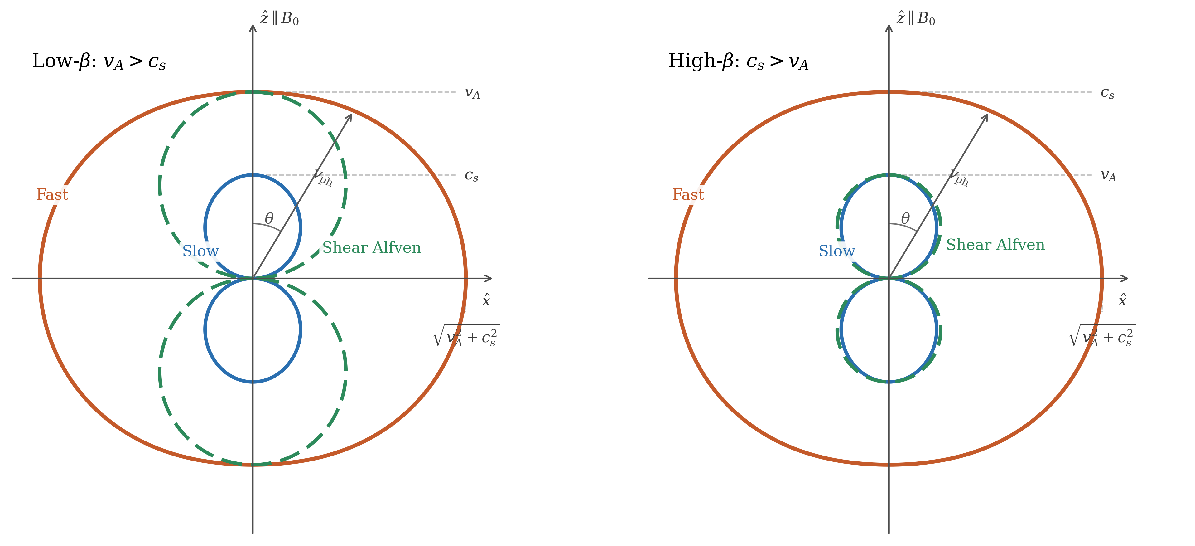
Interactive Alfvén Polar Explorer
Open a browser companion to the lecture’s uniform-wave spectrum. The app scans the slow, shear-Alfvén, and fast branches from low-\(\beta\) to high-\(\beta\), and redraws the polar phase-speed diagram as the pressure ratio \(c_s^2/v_A^2\) changes.
Open the Alfvén polar explorer
Useful limits.
Several limits are worth recording explicitly. If \(k_\parallel =0\), then Eq. (14.18) gives \(\omega =0\), so there is no propagating
shear-Alfvén wave across the field in uniform ideal MHD. If \(k_\perp =0\), the \(x\)–\(z\) block diagonalizes and one recovers a
sound wave \(\omega ^2=c_s^2k_\parallel ^2\) together with the Alfvén wave \(\omega ^2=v_A^2k_\parallel ^2\). In the low-\(\beta \) limit, \(v_A\gg c_s\), the fast mode approaches \(\omega ^2\simeq v_A^2 k^2\), while the slow
mode becomes predominantly acoustic along the field.
Entropy mode.
Besides the propagating branches there is also a zero-frequency entropy mode. The linearized adiabatic law
may be written as
\[-i\omega \left (\frac {p_1}{p_0} - \gamma \frac {\rho _1}{\rho _0}\right )=0. \tag{14.24}\]
If \(\omega =0\), Eqs. (14.4) and (14.6) force \(\uvec _1=\B _1=p_1=0\), but a stationary perturbation of entropy remains possible. This root does
not propagate, but it is part of the full linear spectrum.
Bridge to the Alfvén continuum.
The uniform formula \(\omega ^2=k_\parallel ^2 v_A^2\) is the seed of a much more important result in nonuniform geometry. In a
large-aspect-ratio tokamak,
\[k_\parallel (\psi ) \simeq \frac {n-m/q(\psi )}{R_0}, \tag{14.25}\]
so the local shear-Alfvén relation becomes \[\boxed { \omega ^2 = k_\parallel ^2(\psi )\, v_A^2(\psi ). } \tag{14.26}\]
Each flux surface therefore carries its own natural shear-Alfvén frequency. That surface-by-surface
resonance structure is the Alfvén continuum. Later, when toroidicity couples neighboring poloidal
harmonics, gaps open in this continuum and toroidal Alfvén eigenmodes can live in those
gaps.
Caution
The uniform-plasma calculation is the right starting point, but it does not yet know
about continuum singularities, toroidal coupling, continuum damping, or gap modes.
Those are geometric effects that appear only when \(q(\psi )\), \(B(\psi )\), and \(v_A(\psi )\) vary across the plasma.
14.2 CGL extension of the wave spectrum
The next question is whether the same wave problem survives when the pressure is anisotropic. In the
CGL lecture the equilibrium stress was written as
\[\tens {P}_0 = p_{\perp 0}\,\tens {I} + \left (p_{\parallel 0}-p_{\perp 0}\right )\vect {b}\vect {b}, \tag{14.27}\]
with double-adiabatic closure derived from the invariants \(p_\perp /(nB)=\text {const}\) and \(p_\parallel B^2/n^3=\text {const}\).
Uniform anisotropic equilibrium.
Take the same uniform field geometry,
\[\B _0 = B_0 \vect {e}_z, \qquad \rho _0,p_{\perp 0},p_{\parallel 0}=\text {const}, \qquad \vect {k}=k_\perp \vect {e}_x + k_\parallel \vect {e}_z. \tag{14.28}\]
Define the directional thermal speeds \[c_\perp ^2 \equiv \frac {p_{\perp 0}}{\rho _0}, \qquad c_\parallel ^2 \equiv \frac {p_{\parallel 0}}{\rho _0}. \tag{14.29}\]
Equation (14.8) still holds, so \[\frac {B_{1\parallel }}{B_0} = -i k_\perp \xi _x, \qquad \vect {b}_1 = \frac {\B _{1\perp }}{B_0} = i k_\parallel (\xi _x\vect {e}_x+\xi _y\vect {e}_y). \tag{14.30}\]
Double-adiabatic pressure perturbations.
For a uniform equilibrium, Eulerian and Lagrangian perturbations coincide. Using the two adiabatic
invariants,
\[\frac {p_\perp }{nB}=\text {const}, \qquad \frac {p_\parallel B^2}{n^3}=\text {const}, \tag{14.31}\]
one finds \[\begin{aligned}\frac {p_{\perp 1}}{p_{\perp 0}} &= \frac {B_{1\parallel }}{B_0} - \divergence \vect {\xi }, \\ \frac {p_{\parallel 1}}{p_{\parallel 0}} &= -2\frac {B_{1\parallel }}{B_0} - 3\divergence \vect {\xi }.\end{aligned} \tag{14.32}\]
Now
\[\divergence \vect {\xi } = i\vect {k}\cdot \vect {\xi } = i k_\perp \xi _x + i k_\parallel \xi _z. \tag{14.34}\]
Insert Eq. (14.8) into Eqs. (14.32)–(14.33): \[\begin{aligned}\frac {p_{\perp 1}}{p_{\perp 0}} &= - i k_\perp \xi _x - \left (i k_\perp \xi _x + i k_\parallel \xi _z\right ) = -2 i k_\perp \xi _x - i k_\parallel \xi _z, \\ \frac {p_{\parallel 1}}{p_{\parallel 0}} &= 2 i k_\perp \xi _x - 3\left (i k_\perp \xi _x + i k_\parallel \xi _z\right ) = - i k_\perp \xi _x - 3 i k_\parallel \xi _z.\end{aligned} \tag{14.35}\]
Perturbed pressure tensor.
Write
\[\tens {P}_1 = p_{\perp 1}\,\tens {I} + (p_{\parallel 1}-p_{\perp 1})\,\vect {b}\vect {b} + \left (p_{\parallel 0}-p_{\perp 0}\right )\left (\vect {b}_1\vect {b}+\vect {b}\vect {b}_1\right ). \tag{14.37}\]
Because \(\vect {b}=\vect {e}_z\), the only off-diagonal elements come from \(\vect {b}_1\vect {b}+\vect {b}\vect {b}_1\). Using Eq. (14.30), \[P_{1,xz}=P_{1,zx} = \left (p_{\parallel 0}-p_{\perp 0}\right )i k_\parallel \xi _x, \qquad P_{1,yz}=P_{1,zy} = \left (p_{\parallel 0}-p_{\perp 0}\right )i k_\parallel \xi _y. \tag{14.38}\]
Therefore \[\begin{aligned}(\divergence \tens {P}_1)_x &= i k_\perp p_{\perp 1} - \left (p_{\parallel 0}-p_{\perp 0}\right )k_\parallel ^2\xi _x, \\ (\divergence \tens {P}_1)_y &= - \left (p_{\parallel 0}-p_{\perp 0}\right )k_\parallel ^2\xi _y, \\ (\divergence \tens {P}_1)_z &= i k_\parallel p_{\parallel 1} - \left (p_{\parallel 0}-p_{\perp 0}\right )k_\perp k_\parallel \xi _x.\end{aligned} \tag{14.39}\]
CGL wave matrix.
Collecting the pressure force \(-\divergence \tens {P}_1\) and the magnetic force from Eq. (14.10), one finds
\[\left (\omega ^2 \tens {I} - \tens {K}_{\mathrm {CGL}}\right )\cdot \vect {\xi }=0, \tag{14.42}\]
with \[\boxed { \tens {K}_{\mathrm {CGL}} = \begin {pmatrix} v_A^2 k^2 + 2c_\perp ^2 k_\perp ^2 + (c_\perp ^2-c_\parallel ^2)k_\parallel ^2 & 0 & c_\perp ^2 k_\perp k_\parallel \\[6pt] 0 & k_\parallel ^2\left (v_A^2 + c_\perp ^2-c_\parallel ^2\right ) & 0 \\[6pt] c_\perp ^2 k_\perp k_\parallel & 0 & 3c_\parallel ^2 k_\parallel ^2 \end {pmatrix}. } \tag{14.43}\]
Equivalently, \[\boxed { \omega ^2 \tens {I} - \tens {K}_{\mathrm {CGL}} = \begin {pmatrix} \omega ^2 - v_A^2 k^2 - 2c_\perp ^2 k_\perp ^2 - (c_\perp ^2-c_\parallel ^2)k_\parallel ^2 & 0 & - c_\perp ^2 k_\perp k_\parallel \\[6pt] 0 & \omega ^2 - k_\parallel ^2\left (v_A^2+c_\perp ^2-c_\parallel ^2\right ) & 0 \\[6pt] - c_\perp ^2 k_\perp k_\parallel & 0 & \omega ^2 - 3c_\parallel ^2 k_\parallel ^2 \end {pmatrix}. } \tag{14.44}\]
Anisotropic shear-Alfvén branch.
The \(y\)-polarized mode again decouples:
\[\boxed { \omega ^2 = k_\parallel ^2\left (v_A^2 + c_\perp ^2 - c_\parallel ^2\right ) = k_\parallel ^2 \frac {B_0^2/\muo + p_{\perp 0}-p_{\parallel 0}}{\rho _0}. } \tag{14.45}\]
This is the classic firehose result. The shear branch becomes unstable when \[\boxed { p_{\parallel 0}-p_{\perp 0} > \frac {B_0^2}{\muo }. } \tag{14.46}\]
The physical point is simple and important: pressure anisotropy does not create a new restoring force here;
it subtracts from the old one. The shear branch is controlled by field-line tension, and the firehose
instability appears when that tension changes sign.
Compressional block.
The \(x\)–\(z\) block gives
\[\boxed { \left [ \omega ^2 - \left ( v_A^2 k^2 + 2c_\perp ^2 k_\perp ^2 + (c_\perp ^2-c_\parallel ^2)k_\parallel ^2 \right ) \right ] \left (\omega ^2-3c_\parallel ^2 k_\parallel ^2\right ) - c_\perp ^4 k_\perp ^2 k_\parallel ^2 =0. } \tag{14.47}\]
Expand the first factor using \(k^2=k_\perp ^2+k_\parallel ^2\): \[\begin{aligned}& v_A^2 k^2 + 2c_\perp ^2 k_\perp ^2 + (c_\perp ^2-c_\parallel ^2)k_\parallel ^2 \nonumber \\ &\qquad = k_\perp ^2(v_A^2+2c_\perp ^2) + k_\parallel ^2(v_A^2+c_\perp ^2-c_\parallel ^2).\end{aligned} \tag{14.48}\]
Hence Eq. (14.47) becomes
\[\begin{aligned}0 &= \omega ^4 - \omega ^2 \Bigl [ k_\perp ^2(v_A^2+2c_\perp ^2) + k_\parallel ^2(v_A^2+c_\perp ^2+2c_\parallel ^2) \Bigr ] \nonumber \\ &\qquad + 3c_\parallel ^2 k_\parallel ^2 \Bigl [ k_\perp ^2(v_A^2+2c_\perp ^2) + k_\parallel ^2(v_A^2+c_\perp ^2-c_\parallel ^2) \Bigr ] - c_\perp ^4 k_\perp ^2 k_\parallel ^2 .\end{aligned} \tag{14.49}\]
CGL mirror threshold.
At marginal stability one root passes through \(\omega ^2=0\), so the constant term of Eq. (14.49) must vanish:
\[\begin{aligned}0 &= 3c_\parallel ^2 k_\parallel ^2 \Bigl [ k_\perp ^2(v_A^2+2c_\perp ^2) + k_\parallel ^2(v_A^2+c_\perp ^2-c_\parallel ^2) \Bigr ] - c_\perp ^4 k_\perp ^2 k_\parallel ^2 .\end{aligned} \tag{14.50}\]
The mirror mode is oblique, so \(k_\parallel \neq 0\), and one may divide by \(k_\parallel ^2\):
\[\Bigl [ 3c_\parallel ^2(v_A^2+2c_\perp ^2)-c_\perp ^4 \Bigr ]k_\perp ^2 + 3c_\parallel ^2(v_A^2+c_\perp ^2-c_\parallel ^2)k_\parallel ^2 =0. \tag{14.51}\]
The threshold is first reached in the quasi-perpendicular limit \(k_\parallel /k_\perp \to 0\), so the coefficient of \(k_\perp ^2\) must vanish:
\[c_\perp ^4 = 3c_\parallel ^2(v_A^2+2c_\perp ^2). \tag{14.52}\]
Multiply by \(\rho _0^2\) and restore the pressure variables: \[p_{\perp 0}^2 = 3p_{\parallel 0} \left ( \frac {B_0^2}{\muo }+2p_{\perp 0} \right ). \tag{14.53}\]
Thus the CGL compressive branch becomes unstable when \[\boxed { \frac {p_{\perp 0}^2}{6p_{\parallel 0}} > p_{\perp 0} + \frac {B_0^2}{2\muo }. } \tag{14.54}\]
Caution
Equation (14.54) is historically important, but it is not the final mirror criterion. The
firehose threshold is already correct at the CGL level because it is basically a tension
balance. The mirror mode depends sensitively on the compressive pressure response,
and that is where the kinetic closure matters. The next lecture revisits this same
problem using drift-kinetic pressure perturbations and recovers the standard kinetic
mirror threshold.
Takeaways
The wave lecture teaches three lessons that will matter later.
-
1.
- The shear Alfvén branch, Eq. (14.18), is the cleanest manifestation of magnetic
tension and becomes the Alfvén continuum in nonuniform plasmas.
-
2.
- The fast and slow branches mix magnetic compression with ordinary fluid
compression, and their polarizations are encoded in Eq. (14.23).
-
3.
- Pressure anisotropy does not create a separate theory of waves; it modifies the same
matrix problem. In that language the firehose instability is a sign change of the shear
branch, while the mirror instability belongs to the compressive block and therefore
tests the closure more severely.
Bibliography
Hannes Alfvén. Existence of electromagnetic-hydrodynamic waves. Nature, 150:405–406, 1942. doi:10.1038/150405d0.
S. Lundquist. Experimental investigations of magneto-hydrodynamic waves. Physical Review, 76(12):1805–1809, 1949. doi:10.1103/PhysRev.76.1805.
Bo Lehnert. Magneto-hydrodynamic waves in liquid sodium. Physical Review, 94(4):815–824, 1954. doi:10.1103/PhysRev.94.815.
G. F. Chew, M. L. Goldberger, and F. E. Low. The Boltzmann equation and the one-fluid hydromagnetic equations in the absence of particle collisions. Proceedings of the Royal Society of London. Series A. Mathematical and Physical Sciences, 236(1204):112–118, 1956. doi:10.1098/rspa.1956.0116.
Problems
-
Problem 14.1.
- Starting from Eq. (14.10), derive the matrix (14.15) explicitly. Show every step
in the projection onto the \((x,y,z)\) basis.
-
Problem 14.2.
- Using Eq. (14.23), show that in the low-\(\beta \) limit the slow branch is predominantly
polarized along \(\B _0\), whereas the fast branch is predominantly polarized along \(\vect {k}\).
-
Problem 14.3.
- Derive Eq. (14.26) for a large-aspect-ratio tokamak and explain why a radial
variation of \(q(\psi )\) turns one uniform frequency into a continuum.
-
Problem 14.4.
- Starting from Eqs. (14.35) and (14.36), derive the CGL matrix (14.43). Check
carefully that the field-direction perturbation uses \(\vect {b}_1=\B _{1\perp }/B_0\).
-
Problem 14.5.
- Show directly from Eq. (14.45) that the firehose threshold is equivalent to the
statement that the effective field-line tension changes sign.
-
Problem 14.6.
- Repeat the derivation of the CGL compressive threshold (14.54) and identify
precisely the step where the quasi-perpendicular ordering is used.