Lecture 18
Magnetic Interchange
Interchange modes are the cleanest place to see how equilibrium and stability talk to one another in MHD.
They are the disturbances that try to exchange neighboring flux tubes while doing as little field-line
bending as possible. That makes them the natural magnetic analogue of buoyant overturning, and it is why
the gravitational interchange problem of the previous lecture is such a useful warm-up. In one language the
instability is driven by bad curvature; in another it is governed by the geometry of the volume per unit
flux, usually written as \(V'(\psi )\). Both points of view are useful, and both will reappear later in the ballooning
lecture.
Overview
Big picture. Magnetic interchange is an energy-principle instability. The mode tries to
move plasma across flux surfaces while minimizing magnetic-line bending, so the sign of \(\delta W\)
is controlled primarily by curvature, pressure gradients, and the geometry of the volume
available to a flux tube. In a paraxial mirror this produces the classic flute criterion; in
a more global description it becomes the \(V'(\psi )\) criterion.
Historical Perspective
The classical mirror-interchange problem sits at the beginning of ideal-MHD stability
theory. Kruskal and Schwarzschild first showed how a magnetized plasma can suffer a
buoyancy-like instability even when the magnetic field is frozen into the fluid Kruskal
and Schwarzschild (1954). Rosenbluth and Longmire then made the mirror connection
explicit by interpreting bad magnetic curvature as an effective gravity and by showing
why axisymmetric mirrors are generically vulnerable to flute modes Rosenbluth and
Longmire (1957). Newcomb’s general stability formulation and the energy principle
later placed these arguments on a rigorous variational footing Newcomb (1961). For
mirrors this story remained central for decades, because any serious mirror design had
to contend with interchange from the start: either by creating minimum-\(B\) geometry, by
line-tying the ends, or by weighting the pressure toward good-curvature regions, as in
the sloshing-ion idea of Hinton and Rosenbluth Hinton and Rosenbluth (1982). The
modern axisymmetric treatment by Ryutov et al. is especially useful because it shows
how the classical flute argument survives in a controlled paraxial expansion Ryutov
et al. (2011).
Caution
Where this lecture stops. The interchange mode is the limit in which field-line
bending is minimized. That is why the analysis can be so clean. Once parallel structure
and bending energy become essential, one is already moving toward the ballooning
problem. We therefore keep the focus here on flute-like perturbations and use the lecture
as a bridge between equilibrium, the energy principle, and later ballooning theory.
18.1 Curvature as an Effective Gravity
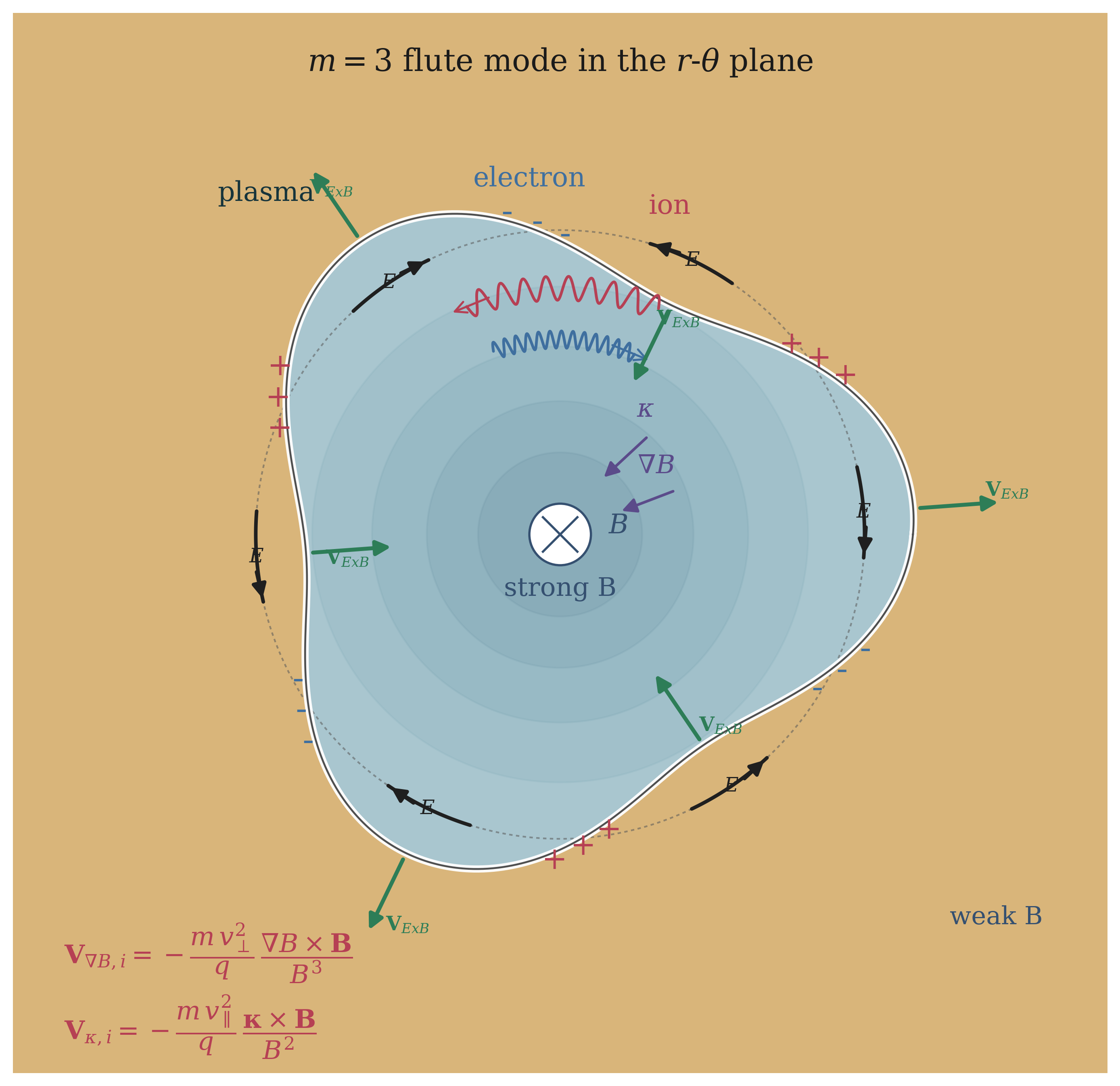
Single-particle picture.
The basic intuition is already visible at the guiding-center level. In a slowly varying magnetic field the
curvature and grad-\(B\) drifts are
\[\vect {v}_d = \frac {1}{qB^2}\, \B \times \left ( m v_\parallel ^2\,\vect {\kappa } + \mu \,\grad B \right ), \tag{18.1}\]
where \[\vect {\kappa } \equiv (\vect {b}\cdot \grad )\vect {b}\]
is the magnetic curvature. For a low-\(\beta \) plasma in which pressure is neglible for equilibrium \[\begin{aligned}\nabla \frac {B^2}{2 \mu _0} & = \frac {B^2}{\mu _0} \vect {\kappa } \\ \nabla B & = B \vect {\kappa }\end{aligned}\]
with approximately thermal perpendicular and parallel energies,
\[\mu B \sim \frac 12 m v_\perp ^2, \qquad m v_\parallel ^2 + \mu B \sim m v_\parallel ^2 + \frac 12 m v_\perp ^2,\]
so Eq. (18.1) suggests the effective acceleration \[\vect {g}_{\rm eff} \sim - \left (v_\parallel ^2 + \frac 12 v_\perp ^2\right )\vect {\kappa } \sim c_s^2\,\vect {\kappa } \sim \frac {c_s^2}{R_{\rm curv}}\,\hat {\vect {R}}. \tag{18.6}\]
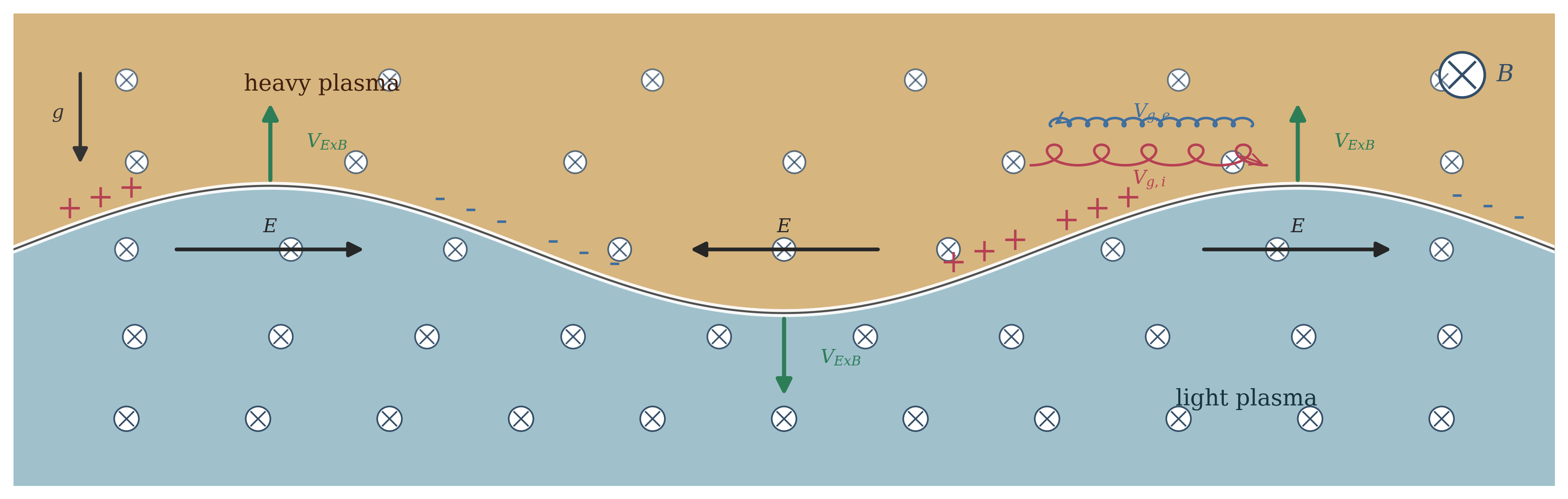
This is the magnetic counterpart of the gravitational acceleration in the previous lecture. Bad curvature
means that the effective gravity points from high pressure toward low pressure, so a pressure gradient can
drive a buoyant interchange exactly as in the Rayleigh–Taylor problem.
The fluid criterion.
The single-particle picture is only a guide, but it points to the correct fluid quantity. When the plasma is
pushed across the field, curvature enters the force balance through the same geometric combination that
appeared in the anisotropic equilibrium lecture, namely \(\vect {\kappa }\cdot \grad p\). The local destabilizing tendency is therefore
\[\vect {\kappa }\cdot \grad p > 0. \tag{18.7}\]
This should be read in parallel with the gravitational criterion of Lecture 16: replace the ordinary
gravity \(\vect g\) by the effective gravity associated with curvature, and the interchange analogy becomes
immediate.
Orbit-averaged drift and pressure weighting.
In a mirror one field line typically contains both good- and bad-curvature regions, so the orbit-averaged
drift matters. For a single particle moving along a field line the net azimuthal displacement over one
bounce is
\[\begin{aligned}\Delta \theta &= \oint \frac {v_{d,\theta }}{r}\,dt = \oint \frac {v_{d,\theta }}{r}\,\frac {d\ell }{v_\parallel } \nonumber \\ &= \oint \frac {\kappa }{qBr} \frac {mv_\parallel ^2 + \frac 12 m v_\perp ^2}{R_c} \frac {d\ell }{v_\parallel } \nonumber \\ &= \oint \sqrt {m} \frac {\kappa }{qBr} \frac { 2 \varepsilon - \mu B \
}{\sqrt {\varepsilon - \mu B}} d\ell\end{aligned} \tag{18.8}\]
Now lets consider the number \(N(\mu ,\varepsilon ) \) on a field line with given \(\mu \) and \(\varepsilon \). The average drift will be \(\langle \Delta \phi \rangle = \int d \mu d\varepsilon N(\mu , \varepsilon ) \Delta \phi (\mu , \varepsilon )\). The distribution
function "density" at any point must vary as
\[f(\mu ,\varepsilon ,\ell ) = k N(\mu ,\varepsilon ) \frac {B}{v_\parallel }\]
where \(k\) is a constant. This follows directly from the real space divergence and the constancy of \(f v_\parallel dA = f \frac {v_\parallel }{B} d\Phi \) in a flux
tube of flux \(d\Phi \).
A distribution function \(f(v_\parallel ,\mu )\) on the other hand, weights different parts of the field line differently, so the
collective drift of a thin flux tube depends on how the pressure is distributed along the orbit. For a small
flux tube of flux \(d\Phi \) the distribution-function average is
\[\begin{aligned}N\,\langle \Delta \theta \rangle &= d \Phi \frac {\sqrt {m}}{q} \int _1^2 d\ell \int d^3v\; f(v_\parallel ,\mu ) \frac {\kappa }{rB^2} \left (mv_\parallel ^2 + \frac 12 m v_\perp ^2\right ) \nonumber \\ &= d \Phi \frac {\sqrt {m}}{q} \int _1^2 d\ell \; \frac {\kappa }{rB^2} \left (p_\parallel + p_\perp \right ).\end{aligned} \tag{18.10}\]
where the limits of integration might span the maximum field in the throat of the mirror where \(\kappa = 0\).
This is the first hint that the combination \(p_\parallel +p_\perp \) and its weighting along the field line will control
the interchange drive. It also explains why highly anisotropic distributions can sometimes
stabilize a nominally bad-curvature mirror by placing pressure in the good-curvature regions
Hinton and Rosenbluth (1982). For isotropic plasmas the stability is governed by the integral
\[\int _1^2 d\ell \; \frac {\kappa }{rB^2}, \tag{18.11}\]
we will return to this later.
18.2 Paraxial Axisymmetric Mirror Geometry
Flux coordinates in a thin mirror.
We now specialize to a paraxial axisymmetric mirror with radial scale \(r\) much smaller than the axial
variation scale \(L\),
\[\epsilon \equiv \frac {r}{L} \ll 1.\]
To lowest order the field is approximately axial, \[\B \simeq B(z)\,\hat {\vect z}, \qquad B=B(z),\]
and the usual axisymmetric flux function satisfies \[2\pi \psi \equiv \int _S \B \cdot d\vect S.\]
For a circle of radius \(r\) this gives \[2\pi \psi \simeq \pi r^2 B(z) \qquad \Longrightarrow \qquad \psi \simeq \frac {B(z)r^2}{2}, \tag{18.15}\]
so the radius of the flux surface \(\psi ={\rm const}\) is \[r(z;\psi ) = \sqrt {\frac {2\psi }{B(z)}}. \tag{18.16}\]
Equation (18.15) is the same paraxial relation used earlier in the anisotropic-equilibrium lecture.
Curvature and normal derivatives.
The field-line curvature is
\[\vect {\kappa } \equiv (\vect b\cdot \grad )\vect b, \qquad \kappa \equiv \vect {\kappa }\cdot \hat {\vect n},\]
where \(\hat {\vect n}\) points outward across the flux surfaces. For a low-\(\beta \) vacuum field, \[\kappa \simeq \frac {1}{B}\pp {B}{n}, \tag{18.18}\]
which is the paraxial form of the more general curvature relations developed in Eq. (9.6). Because
Eq. (18.15) implies \[\pp {}{n} = \pp {\psi }{n}\pp {}{\psi } = rB\pp {}{\psi }, \tag{18.19}\]
Eq. (18.18) may also be written as \[\kappa = -rB^2\pp {}{\psi }\left (\frac {1}{B}\right ). \tag{18.20}\]
Equilibrium identities.
The gyrotropic equilibrium relations derived in Lecture 9 will be used repeatedly below. Parallel balance is
\[\pp {p_\parallel }{\ell } = -\frac {p_\parallel -p_\perp }{B}\pp {B}{\ell }, \tag{18.21}\]
which is Eq. (9.11), and perpendicular balance is \[\pp {}{n}\left (p_\perp + \frac {B^2}{2\muo }\right ) + \kappa \left (p_\parallel -p_\perp -\frac {B^2}{2\muo }\right ) = 0, \tag{18.22}\]
which is the paraxial form of Eq. (9.13). These relations tell us that even before doing any linear stability
analysis, curvature has already entered the equilibrium force balance. The instability problem
asks whether a neighboring flux tube can lower the energy further by exploiting that same
curvature.
18.3 Flute Ordering and the Field-Line-Integrated Equation
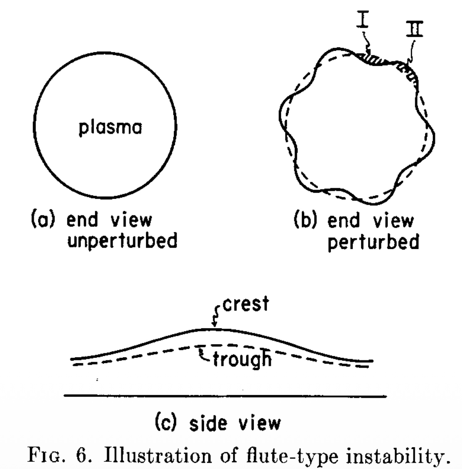
Why flute modes are special.
Interchange modes are characterized by short perpendicular structure and very weak parallel variation.
Write the displacement as
\[\vect \xi (\vect x,t) = \vect \xi (\vect x)\,e^{-i\omega t + i m\theta },\]
with large azimuthal mode number \(m\) and negligible field-line bending to leading order. In a low-\(\beta \) vacuum
equilibrium, \(\J _0 = \curl \B /\muo \simeq 0\), so the linearized momentum equation becomes \[-\omega ^2 \rho \,\vect \xi = \delta \vect f + \delta \J \times \B , \tag{18.24}\]
where \(\delta \vect f \equiv -\divergence \delta \tens P\). This is the same force-balance operator already encountered in the energy-principle lecture, but
now specialized to the flute limit where magnetic bending is deliberately minimized.
Ideal induction and stream function.
The frozen-in condition from Eq. (1.13) gives
\[\delta \B = \curl (\vect \xi \times \B ). \tag{18.25}\]
For the leading flute motion we set \(\delta \B \simeq 0\). Then \[\curl (\vect \xi \times \B )=\vect 0 \qquad \Longrightarrow \qquad \vect \xi \times \B = \grad \varphi , \tag{18.26}\]
for a scalar stream function \(\varphi \). Taking the component along \(\B \) shows that \[\vect b\cdot \grad \varphi = 0, \tag{18.27}\]
so \(\varphi \) is constant along each field line. The perpendicular displacement is therefore \[\vect \xi _\perp = \frac {\B \times \grad \varphi }{B^2}. \tag{18.28}\]
In paraxial cylindrical geometry, \[\xi _n = -\frac {1}{rB}\pp {\varphi }{\theta } = -\frac {i m}{rB}\,\varphi . \tag{18.29}\]
This is the basic kinematic ingredient behind the entire interchange reduction.
Perpendicular current.
Cross Eq. (18.24) with \(\B /B^2\). The parallel part of the pressure force drops out, and one obtains the
perpendicular perturbed current
\[\delta \J _\perp = \omega ^2\rho \,\frac {\B \times \vect \xi }{B^2} + \frac {\B \times \grad \delta p_\perp }{B^2} + (\delta p_\parallel -\delta p_\perp ) \frac {\B \times \vect \kappa }{B^2}. \tag{18.30}\]
Using Eq. (18.26), \[\B \times \vect \xi = \grad \varphi ,\]
so the inertial term is simply proportional to \(\grad \varphi \). Equation (18.30) already exhibits the three pieces of flute
physics: polarization current, diamagnetic response, and curvature coupling.
Current continuity integrated along the field line.
Because charge is conserved,
\[\divergence \delta \J = 0.\]
Write \[\delta \J = \delta J_\parallel \vect b + \delta \J _\perp .\]
Then \[\divergence (\delta J_\parallel \vect b) = B\pp {}{\ell }\left (\frac {\delta J_\parallel }{B}\right ),\]
so integrating along the field line gives \[\left (\frac {\delta J_\parallel }{B}\right )_2 - \left (\frac {\delta J_\parallel }{B}\right )_1 = \int _1^2 \frac {d\ell }{B}\,\divergence \delta \J _\perp . \tag{18.35}\]
This equation is important conceptually. For open or insulating ends the left-hand side vanishes; for
line-tied or conducting ends it is the boundary channel through which the end condition modifies the
interchange spectrum.
Divergence of the inertial term.
Using Eq. (18.30) together with Eq. (18.26),
\[\divergence \delta \J _\perp = \omega ^2\divergence \left (\frac {\rho }{B^2}\grad \varphi \right ) + \divergence \left (\frac {\B }{B^2}\times \grad \delta p_\perp \right ) + \divergence \left [ (\delta p_\parallel -\delta p_\perp ) \frac {\B \times \vect \kappa }{B^2} \right ]. \tag{18.36}\]
The inertial term is the easiest to reduce. In paraxial cylindrical coordinates, \[\begin{aligned}\divergence \left (\frac {\rho }{B^2}\grad \varphi \right ) &\simeq \frac {1}{r}\pp {}{r} \left (\frac {r\rho }{B^2}\pp {\varphi }{r}\right ) + \frac {1}{r^2}\pp {}{\theta } \left (\frac {\rho }{B^2}\pp {\varphi }{\theta }\right ) \nonumber \\ &= \frac {1}{r}\pp {}{r} \left (\frac {r\rho }{B^2}\pp {\varphi }{r}\right ) - \frac {m^2\rho }{r^2B^2}\,\varphi .\end{aligned} \tag{18.37}\]
Now use Eq. (18.15), namely \(r\pp {}{r}=2\psi \pp {}{\psi }\). Then
\[\begin{aligned}\frac {1}{r}\pp {}{r} \left (\frac {r\rho }{B^2}\pp {\varphi }{r}\right ) &= \frac {1}{r}\pp {}{r} \left (\frac {r\rho }{B^2}\,rB\pp {\varphi }{\psi }\right ) \nonumber \\ &= \frac {1}{r}\pp {}{r} \left (\frac {r^2\rho }{B}\pp {\varphi }{\psi }\right ) = \frac {1}{r}\pp {}{r} \left (\frac {2\rho \psi }{B^2}\pp {\varphi }{\psi }\right ) \nonumber \\ &= \frac {2}{B}\pp {}{\psi } \left (\rho \psi \pp {\varphi }{\psi }\right ).\end{aligned}\]
Likewise,
\[\frac {m^2\rho }{r^2B^2}\,\varphi = \frac {m^2\rho }{2\psi B}\,\varphi .\]
Therefore \[\divergence \left (\frac {\rho }{B^2}\grad \varphi \right ) = \frac {2}{B} \left [ \pp {}{\psi }\left (\rho \psi \pp {\varphi }{\psi }\right ) - \frac {m^2\rho }{4\psi }\,\varphi \right ]. \tag{18.40}\]
Pressure contribution.
The pressure terms can also be reduced explicitly. Using
\[\divergence (\vect A\times \vect C) = \vect C\cdot \curl \vect A - \vect A\cdot \curl \vect C,\]
with \(\vect A = \B /B^2\) and \(\vect C = \grad \delta p_\perp \) gives \[\divergence \left (\frac {\B }{B^2}\times \grad \delta p_\perp \right ) = \curl \left (\frac {\B }{B^2}\right )\cdot \grad \delta p_\perp ,\]
since \(\curl \grad \delta p_\perp = \vect 0\). For a vacuum field, \[\curl \left (\frac {\B }{B^2}\right ) = \grad \left (\frac {1}{B^2}\right )\times \B = \frac {2\B \times \grad B}{B^3},\]
so in paraxial geometry \[\divergence \left (\frac {\B }{B^2}\times \grad \delta p_\perp \right ) = \frac {2}{rB^2}\pp {B}{n}\pp {\delta p_\perp }{\theta }. \tag{18.44}\]
Similarly, \[\begin{aligned}\divergence \left [ (\delta p_\parallel -\delta p_\perp ) \frac {\B \times \vect \kappa }{B^2} \right ] &= \frac {1}{rB^2}\pp {B}{n}\pp {}{\theta } \left (\delta p_\parallel -\delta p_\perp \right ).\end{aligned} \tag{18.45}\]
Adding Eqs. (18.44) and (18.45) gives the compact result
\[\divergence \left (\frac {\B }{B^2}\times \grad \delta p_\perp \right ) + \divergence \left [ (\delta p_\parallel -\delta p_\perp ) \frac {\B \times \vect \kappa }{B^2} \right ] = \frac {1}{rB^2}\pp {B}{n}\pp {}{\theta } \left (\delta p_\parallel +\delta p_\perp \right ). \tag{18.46}\]
The interchange mode therefore depends only on the combination \[P_\Sigma \equiv p_\parallel + p_\perp .\]
Advection of the pressure sum.
Because flute motion moves an entire thin flux tube sideways with little parallel rearrangement, the leading
perturbation of \(P_\Sigma \) is simply the sideways advection of the equilibrium profile:
\[\delta P_\Sigma \simeq -\xi _n\pp {P_\Sigma }{n}. \tag{18.48}\]
Using Eq. (18.29) and then Eq. (18.19), \[\begin{aligned}\delta P_\Sigma &= -\left (-\frac {i m}{rB}\varphi \right )\pp {P_\Sigma }{n} \nonumber \\ &= \frac {i m}{rB}\varphi \,\pp {P_\Sigma }{n} = i m\varphi \,\pp {P_\Sigma }{\psi }.\end{aligned} \tag{18.49}\]
Substituting Eq. (18.49) into Eq. (18.46) and using \(\pp {B}{n}=\kappa B\) gives
\[\text {pressure terms} = - m^2\,\frac {\kappa }{rB}\,\pp {P_\Sigma }{\psi }\,\varphi . \tag{18.50}\]
This is the local curvature-drive term. It has exactly the sign one expects: outward-decreasing pressure
together with bad curvature is destabilizing.
Field-line-integrated eigenvalue equation.
Insert Eqs. (18.40) and (18.50) into Eq. (18.35). Because \(\varphi \) is constant along the field line, all \(z\)-dependence
sits inside the line integrals. Define
\[\begin{aligned}I(\psi ) &\equiv \int _1^2 \frac {\rho (\psi ,\ell )}{2B^2(\psi ,\ell )}\,d\ell , \\[0.5em] D(\psi ) &\equiv -\int _1^2 \frac {\kappa (\psi ,\ell )}{r(\psi ,\ell )B^2(\psi ,\ell )} \pp {P_\Sigma }{\psi }(\psi ,\ell ) \,d\ell .\end{aligned} \tag{18.51}\]
Then the flute equation becomes
\[i\omega \left [ \left (\frac {\delta J_\parallel }{B}\right )_2 - \left (\frac {\delta J_\parallel }{B}\right )_1 \right ] = \omega ^2 \left [ 4\pp {}{\psi }\left (I\psi \pp {\varphi }{\psi }\right ) - \frac {m^2 I}{\psi }\,\varphi \right ] - m^2 D\,\varphi . \tag{18.53}\]
Equation (18.53) is the paraxial mirror interchange equation. It is the mirror analogue of the
energy-principle form encountered in the previous two lectures: an inertial denominator weighted by \(I(\psi )\) and a
drive weighted by the curvature integral \(D(\psi )\). With the sign convention of Eq. (18.52), bad curvature and an
outward-decreasing \(P_\Sigma \) give \(D>0\).
18.4 Variational Form, Sharp-Boundary Mirrors, and Pressure Weighting
Open ends and the variational principle.
For insulating or effectively open ends,
\[\left (\frac {\delta J_\parallel }{B}\right )_1 = \left (\frac {\delta J_\parallel }{B}\right )_2 = 0,\]
so the left-hand side of Eq. (18.53) vanishes. Multiply the remaining equation by \(\varphi ^*(\psi )\) and integrate from the
axis to the plasma edge. Assuming the boundary terms vanish, \[\begin{aligned}0 &= \omega ^2 \int d\psi \; \varphi ^* \left [ 4\pp {}{\psi }\left (I\psi \pp {\varphi }{\psi }\right ) - \frac {m^2 I}{\psi }\,\varphi \right ] - m^2\int d\psi \;D|\varphi |^2 \nonumber \\ &= -\omega ^2 \int d\psi \; \left [ 4 I\psi \left |\pp {\varphi }{\psi }\right |^2 + \frac {m^2 I}{\psi }|\varphi |^2 \right ] - m^2\int d\psi \;D|\varphi |^2.\end{aligned}\]
Therefore
\[\omega ^2 = - m^2 \frac {\displaystyle \int d\psi \;D(\psi )|\varphi |^2} {\displaystyle \int d\psi \;\left [ 4I(\psi )\psi \left |\pp {\varphi }{\psi }\right |^2 + \frac {m^2 I(\psi )}{\psi }|\varphi |^2 \right ]}. \tag{18.56}\]
This is an energy principle in the same spirit as Eq. (13.18). The denominator is positive definite, so
instability requires \[\int d\psi \;D(\psi )|\varphi |^2 > 0.\]
The flute mode is therefore unstable whenever the weighted bad-curvature drive dominates.
Local high-\(m\) form.
If the mode is radially localized, the derivative term in Eq. (18.56) is subdominant and the local dispersion
relation becomes
\[\begin{aligned}\omega ^2 & \simeq -\frac {\psi D(\psi )}{I(\psi )} \nonumber \\ & \sim \frac {B r^2 \frac {\kappa }{r\cancel {B^2} } \frac {\partial p}{\partial r } \frac {\partial r}{\partial \psi } \cancel {L}}{\frac {\rho }{2 \cancel {B^2} \cancel {L} }} \nonumber \\ & \sim \frac {\frac { p}{L_p}}{R_{curv} \rho }\nonumber \\ & \sim \frac {v_{Ti}^2}{r R_{curv}} \nonumber \\ &\sim \frac {g}{L_p}\end{aligned}\]
This is the simplest statement of the flute instability. A positive \(D\) gives \(\omega ^2<0\), hence pure exponential
growth. Recall the Brunt–Väisälä frequency \(N^2 \sim g / L_p \). The tendency of the fastest ideal modes to run
to short perpendicular wavelength is one reason finite-Larmor-radius physics later becomes
important. We will return to that regularization in the Roberts–Taylor and anisotropic-wave
lectures.
Sharp-boundary mirror.
The sign of \(D\) is especially transparent when the pressure falls sharply to zero at the last closed surface. Let
the plasma edge be \(r=a(z)\) on the flux surface \(\psi =\psi _a\). Since Eq. (18.15) gives \(B(z)a^2(z)=2\psi _a\), one has
\[\frac {1}{aB^2} = \frac {a^3}{4\psi _a^2}.\]
For a vacuum paraxial field the boundary curvature is approximately \[\kappa \simeq -\dd {^2 a}{z^2}.\]
If \(P_\Sigma \) is constant on the field line and drops to zero across a thin edge layer, then Eq. (18.52) gives
\[D_{\rm edge} \propto -\int _1^2 a^3(z)\dd {^2 a}{z^2}\,dz\;[P_\Sigma ], \tag{18.61}\]
where \([P_\Sigma ]\) is the pressure jump across the edge. Integrating by parts, \[\begin{aligned}-\int _1^2 a^3\dd {^2 a}{z^2}\,dz &= -\left [a^3\dd {a}{z}\right ]_1^2 + 3\int _1^2 a^2\left (\dd {a}{z}\right )^2dz.\end{aligned}\]
At the turning points of a symmetric mirror \(da/dz=0\), so the boundary term vanishes and
\[-\int _1^2 a^3\dd {^2 a}{z^2}\,dz = 3\int _1^2 a^2\left (\dd {a}{z}\right )^2dz >0. \tag{18.63}\]
Thus an isotropic sharp-boundary axisymmetric mirror is generically interchange unstable. This is one of
the classical reasons simple mirrors are so unforgiving.
Pressure weighting and sloshing ions.
The same calculation also shows how anisotropy or energetic trapped populations can help. Suppose the
pressure weighting along the field line is \(P_\Sigma =P_\Sigma (a)\) rather than a constant. Then
\[D \propto -\int _1^2 P_\Sigma (a)\,a^3\dd {^2 a}{z^2}\,dz.\]
Integrating by parts again gives \[\begin{aligned}D &= -\left [P_\Sigma a^3 \dd {a}{z}\right ]_1^2 + \int _1^2 \dd {a}{z}\,\dd {}{z}\left (P_\Sigma a^3\right )dz \nonumber \\ &= \int _1^2 \left (\dd {a}{z}\right )^2 \dd {}{a}\left (P_\Sigma a^3\right )dz.\end{aligned} \tag{18.65}\]
For ordinary isotropic pressure, \(\dd {}{a}(P_\Sigma a^3)>0\) and the mode remains unstable. Stability demands instead that
\[\dd {}{a}\left (P_\Sigma a^3\right ) < 0, \tag{18.66}\]
which means that the pressure must be concentrated strongly enough in the good-curvature regions. This
is the logic behind sloshing-ion stabilization Hinton and Rosenbluth (1982).
End conditions and partial line-tying.
Equation (18.35) also shows how end conditions modify the instability. For a high-\(m\) localized mode we may
drop the radial-derivative term in Eq. (18.53), obtaining
\[i\omega \left [ \left (\frac {\delta J_\parallel }{B}\right )_2 - \left (\frac {\delta J_\parallel }{B}\right )_1 \right ] = -\omega ^2\frac {m^2 I}{\psi }\,\varphi - m^2 D\,\varphi . \tag{18.67}\]
If each end is connected to a sheath or limiter with small-signal impedance \(Z_{\rm sh}\), then the linearized end
response can be modeled as \[\delta J_{\parallel ,2} = +\frac {\varphi }{Z_{\rm sh}}, \qquad \delta J_{\parallel ,1} = -\frac {\varphi }{Z_{\rm sh}}. \tag{18.68}\]
For a symmetric mirror with end field \(B_{\rm end}\), \[\left (\frac {\delta J_\parallel }{B}\right )_2 - \left (\frac {\delta J_\parallel }{B}\right )_1 = \frac {2\varphi }{B_{\rm end}Z_{\rm sh}}. \tag{18.69}\]
Substituting into Eq. (18.67) yields \[\omega ^2 + i\Gamma _{\rm LT}\omega + \Gamma _0^2 = 0, \tag{18.70}\]
with \[\Gamma _0^2 \equiv \frac {\psi D}{I}, \qquad \Gamma _{\rm LT} \equiv \frac {2\psi }{m^2 I B_{\rm end} Z_{\rm sh}}. \tag{18.71}\]
For open ends \(\Gamma _{\rm LT}=0\) and one recovers \(\omega ^2=-\Gamma _0^2\). For strong line-tying, \(\Gamma _{\rm LT}\gg \Gamma _0\), the growth rate becomes \[\gamma \simeq \frac {\Gamma _0^2}{\Gamma _{\rm LT}}, \tag{18.72}\]
so line-tying does not change the ideal drive itself but can make the mode arbitrarily slow by providing the
parallel current needed to short out the flute polarization.
18.5 A Second Energy Principle: the \(V'(\psi )\) Criterion
Why a second formulation is useful.
The mirror calculation above emphasizes local curvature and current continuity. There is, however, a more
geometric way to express the same interchange physics. If the displacement really does exchange
neighboring flux tubes with very little field-line bending, then the central quantity is the volume available
to a tube of given flux. This is the origin of the \(V'(\psi )\) criterion. It is especially useful because it
makes the instability look transparently like a buoyancy problem in a nontrivial magnetic
geometry.
Volume per unit flux.
For an axisymmetric flux surface labeled by \(\psi \), let \(V(\psi )\) be the volume enclosed by that surface. A thin shell
between \(\psi \) and \(\psi +d\psi \) has volume
\[dV = 2\pi \,d\psi \oint \frac {d\ell }{B},\]
so \[V'(\psi ) \equiv \frac {dV}{d\psi } = 2\pi \oint \frac {d\ell }{B}. \tag{18.74}\]
Up to the conventional factor \(2\pi \), the same geometric content is carried by \[U(\psi ) \equiv \oint \frac {d\ell }{B}. \tag{18.75}\]
The prime notation is traditional in equilibrium theory, so in this lecture it is natural to emphasize
\(V'(\psi )\).
Flux-Tube Derivation of the Marginal Pressure Profile
The flux-tube argument used in the main text is worth writing out in full. Take a tube of flux \(d\psi \) with volume
\(d V = V'(\psi )d\psi \). Adiabatic transport implies
\[p(\psi )\,[V'(\psi )]^\gamma = p_\star (\psi +d\psi )\,[V'(\psi +d\psi )]^\gamma .\]
Therefore \[p_\star (\psi +d\psi ) = p(\psi ) \left [ \frac {V'(\psi )}{V'(\psi +d\psi )} \right ]^\gamma .\]
Expanding \[V'(\psi +d\psi )=V'(\psi )+\frac {d V'}{d\psi }d\psi ,\]
we have \[\begin{aligned}\left [\frac {V'(\psi )}{V'(\psi +d\psi )}\right ]^\gamma &= \left [ 1+\frac {1}{V'}\frac {d V'}{d\psi }d\psi \right ]^{-\gamma } \nonumber \\ &\simeq 1-\gamma \frac {1}{V'}\frac {d V'}{d\psi }d\psi .\end{aligned}\]
Hence
\[p_\star (\psi +d\psi ) \simeq p(\psi ) \left [ 1-\gamma \frac {1}{V'}\frac {d V'}{d\psi }d\psi \right ].\]
The ambient pressure at the new location is \[p(\psi +d\psi ) = p(\psi )+\frac {d p}{d\psi }d\psi .\]
Marginal stability means \(p_\star (\psi +d\psi )=p(\psi +d\psi )\), so \[\frac {d p}{d\psi } = -\gamma \frac {p}{V'}\frac {d V'}{d\psi }.\]
Dividing by \(p\) gives \[\frac {d\ln p}{d\psi } = -\gamma \frac {d\ln V'}{d\psi },\]
or \[p(\psi )\,[V'(\psi )]^\gamma = \mathrm {const}.\]
In terms of a midplane radius label \(r_0\), \[L_{p,\mathrm {crit}} \equiv -\frac {p}{\frac {dp}{d r_0}} = \frac {V'}{\gamma \, \frac {dV'}{d r_0}}.\]
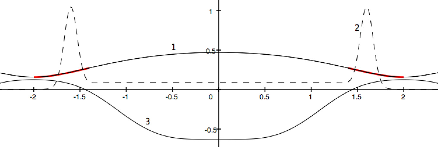
Interchanging two neighboring tubes.
Consider two thin neighboring flux tubes carrying the same infinitesimal flux \(d\Phi \) and centered at \(\psi \) and \(\psi +d\psi \). Their
volumes are
\[V_1 = U(\psi )\,d\Phi , \qquad V_2 = \left [U(\psi )+\pp {U}{\psi }d\psi \right ]d\Phi =\left [U(\psi )+\delta U \right ]d\Phi ,\]
and their pressures are \[p_1 = p(\psi ) = p, \qquad p_2 = p(\psi )+\pp {p}{\psi }d\psi = p + \delta p\]
Now interchange the two tubes. Each tube preserves its entropy, so the pressure of tube 1 after it occupies
the volume \(V_2\) is \[p_1' = p_1\left (\frac {V_1}{V_2}\right )^\gamma ,\]
and similarly \[p_2' = p_2\left (\frac {V_2}{V_1}\right )^\gamma .\]
The thermal energy before the interchange is \[W_i = \frac {p_1V_1}{\gamma -1} + \frac {p_2V_2}{\gamma -1},\]
and after the interchange it is \[W_f = \frac {p_1'V_2}{\gamma -1} + \frac {p_2'V_1}{\gamma -1}.\]
Expanding to second order in \(d\psi \) gives \[\begin{aligned}\Delta W \equiv W_f-W_i & = \delta p \delta U + \gamma p \frac {(\delta U)^2}{U} \\& = (d\psi )^2 \frac {d}{d\psi }\ln \left [p\,U^\gamma \right ].\end{aligned} \tag{18.92}\]
Since \(V'(\psi )=2\pi U(\psi )\) differs only by a constant factor, this may be written equally well as
\[\Delta W \propto \frac {d}{d\psi }\ln \left [p\,\bigl (V'(\psi )\bigr )^\gamma \right ]. \tag{18.94}\]
This is the geometric interchange energy principle. The role of \(V'(\psi )\) is completely analogous to the role of
density stratification in ordinary buoyancy. Since the second term in Eq. (18.92) is manifestly positive, a
sufficient condition for stability is that \[\pp {p}{\psi } \pp {V'}{\psi } > 0\]
which in the general case in which \(p\) decreases outward requires the \(V'\) also decrease outward.
We can come to this same conclusion by returning to the particle drift picture. Combining the stability
integral Eq. (18.11) and the expression for \(\kappa \) from Eq. (18.20), the stability integral requires
\[\int _1^2 \frac {\kappa }{rB^2} d\ell = \int _1^2 d\ell \frac {\partial }{\partial \psi } \frac {1}{B} = \frac {\partial }{\partial \psi } \int _1^2 \frac {d\ell }{B} > 0.\]
For the plasma to gain outward directed energy, the volume must expand.
Stability criterion.
The equilibrium is stable to such an interchange if \(\Delta W>0\). Thus a sufficient instability condition is
\[\frac {d}{d\psi }\ln \left [p\,\bigl (V'(\psi )\bigr )^\gamma \right ] < 0 \qquad \text {when } V''(\psi )>0. \tag{18.97}\]
Equivalently, \[\frac {1}{p}\pp {p}{\psi } + \gamma \,\frac {1}{V'(\psi )}\pp {V'(\psi )}{\psi } < 0. \tag{18.98}\]
This is exactly the same kind of statement as the gravitational energy principle: a sufficiently steep
pressure gradient can overturn the magnetic buoyancy supplied by the geometry.
Straight-current geometry.
For a straight current channel the field is approximately
\[B_\theta = \frac {\muo I}{2\pi r}.\]
A magnetic field line is a circle of circumference \(2\pi r\), so \[U(r) = \oint \frac {d\ell }{B} = \frac {2\pi r}{B_\theta } \propto r^2,\]
and therefore \[V'(r) \propto r^2. \tag{18.101}\]
Then Eq. (18.98) becomes \[\frac {1}{p}\dd {p}{r} + \frac {2\gamma }{r} < 0.\]
Defining the pressure scale length \[L_p \equiv -\frac {p}{dp/dr},\]
one obtains the familiar estimate \[L_p > \frac {r}{2\gamma } \tag{18.104}\]
for marginal interchange stability. This is the same z-pinch intuition encountered from the local curvature
point of view, but expressed in the cleaner geometric language of \(V'(\psi )\). This will be revisited in Lecture
23.
Dipole geometry and self-organization.
The \(V'(\psi )\) language is especially attractive in a dipole, where the flux geometry strongly expands outward.
Dipoles can come in an open-field line geometry like for planets but also in closed-field line geometries like
levitated dipoles. Assuming for now an axisymmetric point dipole moment \(m\) (perhaps suitable for
magnetospheres),
\[\psi (r,\theta ) = r A_\phi = \frac {\muo m\sin ^2\theta }{4\pi r},\]
with spherical coordinates \(r,\theta ,\phi \) A straightforward volume integral gives \[V(\psi ) \propto R^3, \qquad V'(\psi ) \propto R^4, \tag{18.106}\]
where \(R\) is the equatorial crossing radius of each field line. Equation (18.98) then implies that the real space
gradient of pressure in the equatorial plane is governed by \[\frac {1}{p}\dd {p}{R} + \frac {4\gamma }{R} < 0.\]
Marginality therefore gives \[p(R) \propto R^{-4\gamma }. \tag{18.108}\]
For a monatomic gas, \(\gamma =5/3\), so \[p(R) \propto R^{-20/3}.\]
This is a strong profile, but it carries an important physical message: interchange mixing can self-organize
a plasma toward a nearly marginal state, just as ordinary convection tends to drive a stratified atmosphere
toward \(N^2\approx 0\).
Entropy mixing and marginality.
The same dipole example makes another point. If interchange turbulence mixes flux tubes
efficiently, it is natural to expect not only pressure but particle content per unit flux to relax. If
\[\rho V' = \text {const},\]
then \[\frac {1}{\rho }\dd {\rho }{R} + \frac {1}{V'}\dd {V'}{R} =0.\]
Combining this with the marginal pressure profile yields \[\dd {}{R}\left (\frac {p}{\rho ^\gamma }\right )=0,\]
so the entropy becomes approximately flat in radius. That is precisely the magnetic analogue of the way
ordinary convection mixes an atmosphere toward constant entropy.
How the two formulations fit together.
The local \(D(\psi )\) formulation and the global \(V'(\psi )\) formulation are not competitors. They are two views of the same
ideal-MHD interchange physics. The \(D(\psi )\) form is better for paraxial mirrors, end conditions, and pressure
weighting along the field line. The \(V'(\psi )\) form is better for seeing the underlying geometry and for making
contact with the energy principle. In later lectures the ballooning problem will inherit both viewpoints: a
local curvature drive and a global statement about how neighboring flux tubes gain or lose accessible
volume.
Takeaways
Takeaway. Interchange modes are ideal-MHD buoyancy modes. They minimize field-line
bending, so their stability is decided by curvature, pressure gradients, and flux-tube
geometry. In a paraxial mirror the drive is encoded in the field-line integral \(D(\psi )\); in a
more geometric language it is encoded in \(V'(\psi )\). Simple axisymmetric mirrors are therefore
generically unstable, and classical mirror stabilization strategies—minimum-\(B\) design,
pressure weighting, and line-tying—can all be understood as ways of changing the sign
or effectiveness of the same interchange energy principle.
18.6 Bonus: Non-Paraxial, Interchange-Stable Axisymmetric Mirrors
From paraxial intuition to the full flux geometry.
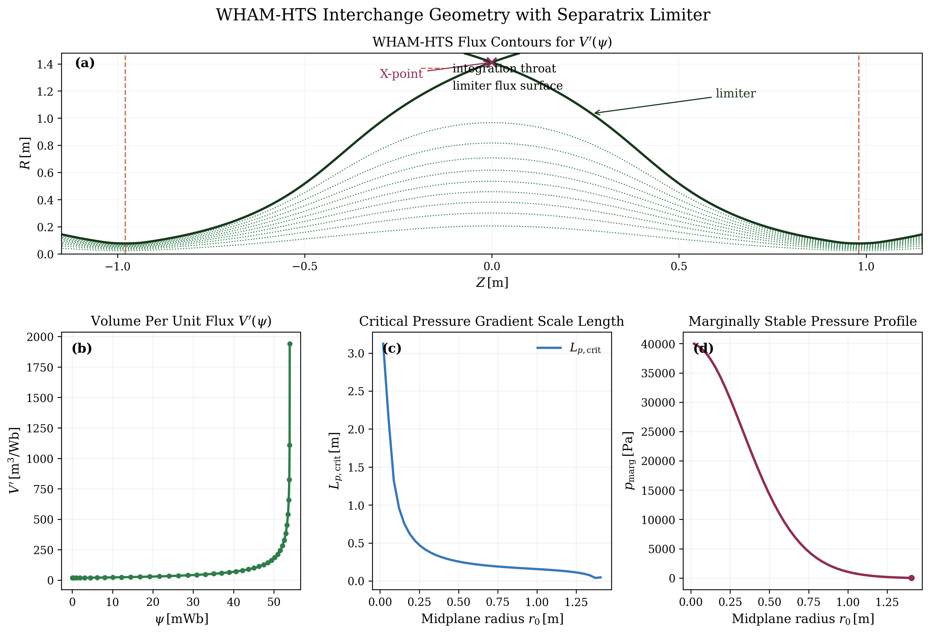
The paraxial mirror analysis is useful for building intuition, but the WHAM geometry is better described
by the exact flux-tube volume per unit flux,
\[V'(\psi )=2\pi \oint \frac {d\ell }{B},\]
evaluated on the axisymmetric vacuum flux surfaces generated by the HTS mirror coils. In this
non-paraxial treatment the outermost relevant surface is not chosen from a small-radius expansion,
but from the separatrix itself. For the present WHAM coil set the midplane null occurs at
\[R_X \simeq 1.412~\mathrm {m},\]
and we take the separatrix flux \(\psi _{\mathrm {sep}}=\psi (R_X,0)\) as the natural limiting surface.
Interchange criterion.
The geometric interchange condition may be written as
\[\frac {1}{p}\pp {p}{\psi } + \gamma \frac {1}{V'}\pp {V'}{\psi } < 0,\]
or, in terms of the midplane radius label \(r_0\), \[L_{p,\mathrm {crit}}(r_0) = \frac {V'}{\gamma \, \dd {V'}{r_0}}.\]
The important point is that the exact WHAM flux geometry produces a very rapid increase in \(V'(\psi )\) as the
separatrix is approached. That geometric expansion strongly relaxes the pressure-gradient constraint
compared with the paraxial-core estimate.
A hot-ion edge state.
To illustrate a non-paraxial WHAM case with a controlled core beta, we choose an edge state just inside
the separatrix with
\[n_{\mathrm {edge}} = 1.0\times 10^{17}~\mathrm {m^{-3}}, \qquad T_{e,\mathrm {edge}} = 12.3~\mathrm {eV}, \qquad T_{i,\mathrm {edge}} = 123.0~\mathrm {eV},\]
so that \[T_e:T_i = 1:10, \qquad p_{\mathrm {edge}} \simeq 2.17~\mathrm {Pa}.\]
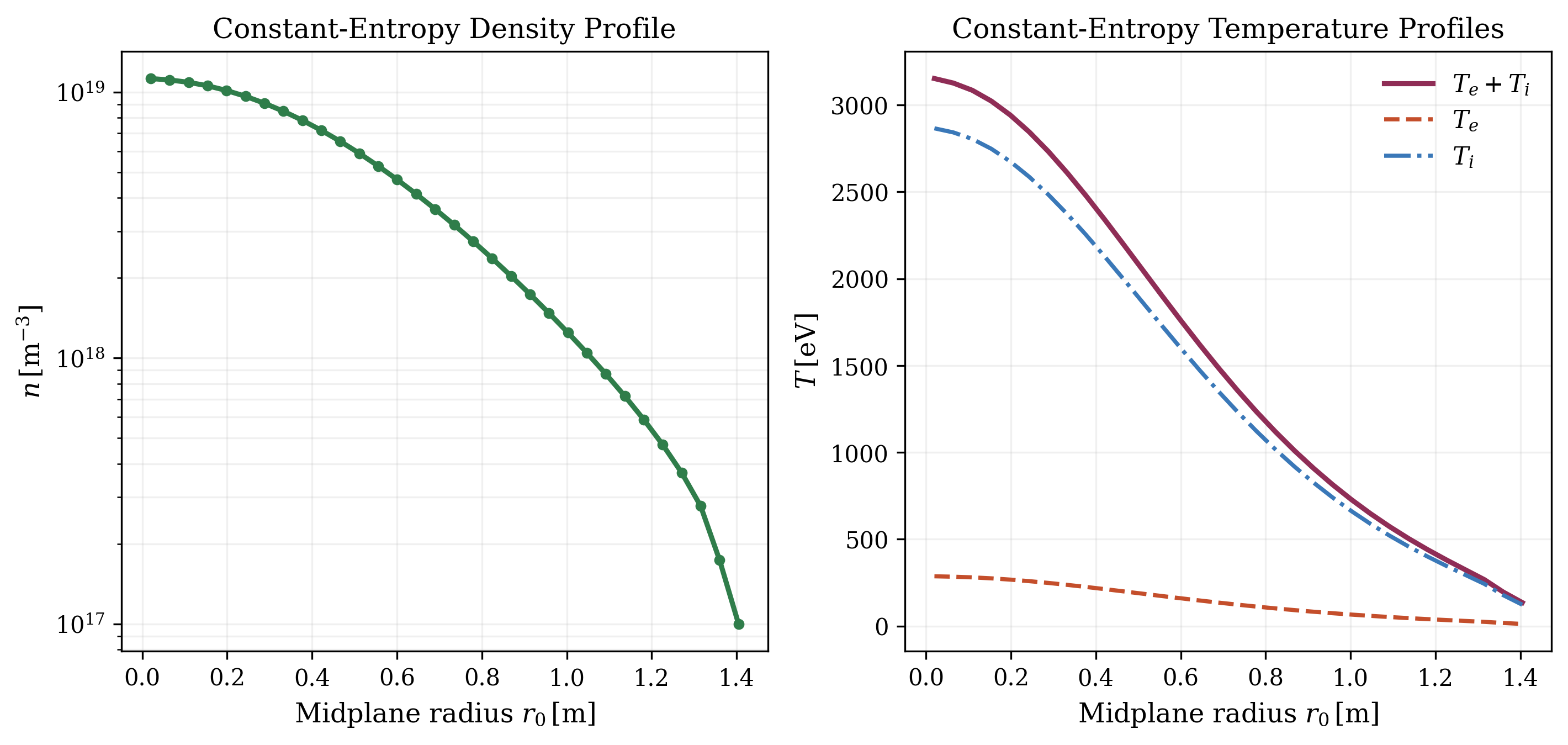
We then integrate the marginal profile inward from the separatrix-limited edge using \[\dd {}{r_0}\ln p = -\frac {1}{L_{p,\mathrm {crit}}}.\]
To close the thermodynamics we additionally assume constant entropy, \[\frac {p}{n^\gamma }=\mathrm {const}, \qquad \gamma =\frac {5}{3},\]
and preserve the electron-to-ion temperature ratio throughout the profile.
What the profiles show.
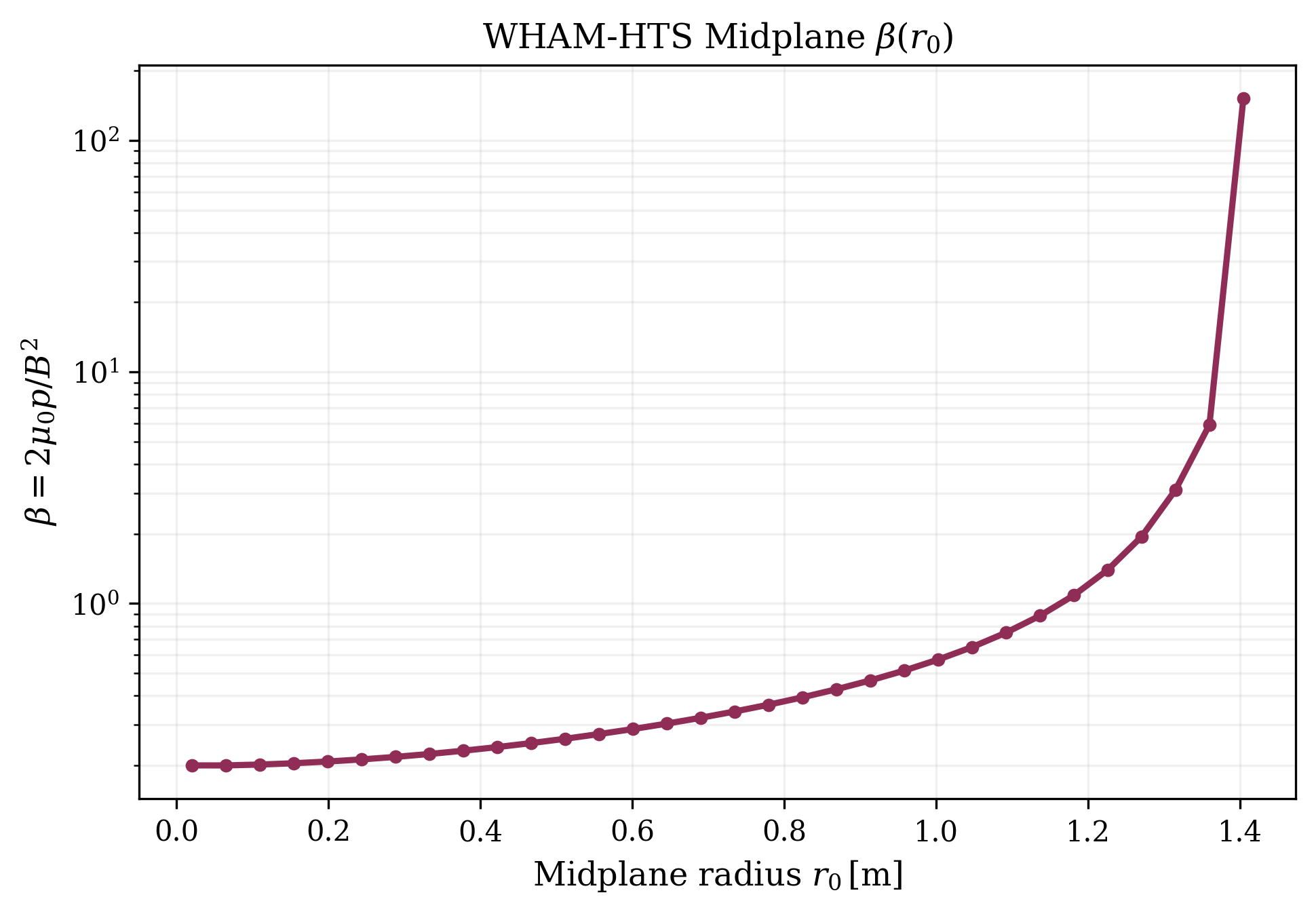
The resulting pressure profile remains modest in the core even though the geometric expansion near the
separatrix is very strong. At the first sampled core point, \(r_0=0.02~\mathrm {m}\), the profile gives
\[\beta (0)\approx 0.20, \qquad \beta (r_0\approx 1~\mathrm {m})\approx 0.57.\]
Thus the core and much of the mid-radius region remain in a regime where an MHD discussion based on
the vacuum flux geometry is at least qualitatively sensible. The same run gives \[n(0.02~\mathrm {m}) \simeq 1.12\times 10^{19}~\mathrm {m^{-3}},\]
with hot-ion temperatures \[T_e(0.02~\mathrm {m}) \simeq 2.87\times 10^2~\mathrm {eV}, \qquad T_i(0.02~\mathrm {m}) \simeq 2.87\times 10^3~\mathrm {eV}.\]
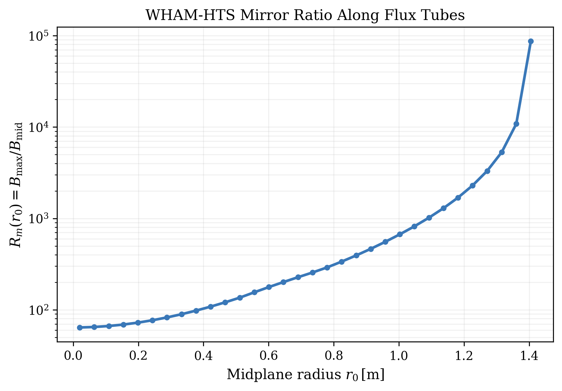
Meanwhile the line-wise mirror ratio grows from about \[R_m \simeq 64\]
on axis to \[R_m \gtrsim 8\times 10^4\]
just inside the separatrix, reflecting the collapse of the midplane field near the null.
Interpretation.
This non-paraxial construction shows that the exact \(V'(\psi )\) geometry of WHAM can support a much larger
pressure buildup than one would infer from a purely paraxial estimate, while still allowing the core beta to
remain below unity for a suitably chosen edge state. That is encouraging from the standpoint of
interchange stability. At the same time, the very large values of \(V'\), mirror ratio, and \(\beta \) as the separatrix is
approached are a warning sign: the outermost flux surfaces lie in a region where the vacuum
field is becoming singular and the magnetic geometry is highly sensitive to finite-pressure
corrections.
What comes next.
For that reason this section should be viewed as a geometric and thermodynamic guide, not as the final
equilibrium solution. The next step is to compute the full high-\(\beta \) MHD equilibrium and revisit
the flux geometry self-consistently. That will determine how much of the large non-paraxial
stabilization survives once the pressure modifies the field rather than simply filling a fixed vacuum
geometry.
Interactive Mirror-Equilibrium Explorer
Open a browser companion to the end of the magnetic-interchange lecture. The app starts from a fixed flux geometry, computes the flux-tube volume per unit flux \(V\prime(\psi)\) or \(U(\psi)=V\prime/(2\pi)\), then integrates the marginal pressure profile inward from a chosen edge pressure. The first version includes a sampled nonparaxial WHAM geometry and an analytic dipole model so you can see how outward field-line expansion relaxes the interchange bound.
Open the mirror-equilibrium explorer
This version keeps the magnetic geometry fixed on purpose. The next step toward a self-consistent anisotropic equilibrium is to loop the pressure back into the field solve with a Picard iteration.
Takeaways
The mirror-interchange lecture has two complementary morals. In the paraxial problem
the drive is encoded in the orbit-weighted curvature integral \(D(\psi )\), which makes clear why
simple axisymmetric mirrors are generically interchange unstable and why line-tying or
pressure weighting can help. In the non-paraxial WHAM geometry the same physics is
reorganized by the exact flux-tube volume \(V'(\psi )\): strong separatrix expansion can greatly relax
the marginal pressure-gradient bound, but only until finite-\(\beta \) corrections to the magnetic
geometry become unavoidable.
Bibliography
M. D. Kruskal and M. Schwarzschild. Some instabilities of a completely ionized plasma. Proceedings of the Royal Society of London A, 223:348–360, 1954. doi:10.1098/rspa.1954.0120.
M.N Rosenbluth and C.L Longmire. Stability of plasmas confined by magnetic fields. Annals of Physics, 1(2):120–140, 1957. doi:10.1016/0003-4916(57)90055-6.
W. A. Newcomb. Convective instability induced by gravity in a plasma with a frozen-in magnetic field. Physics of Fluids, 4:391–396, 1961. doi:10.1063/1.1706342.
F L Hinton and M N Rosenbluth. Stabilization of axisymmetric mirror plasmas by energetic ion injection. Nuclear Fusion, 22(12):1547–1557, 1982. doi:10.1088/0029-5515/22/12/001.
D D Ryutov, H L Berk, B I Cohen, A W Molvik, and T C Simonen. Magneto-hydrodynamically stable axisymmetric mirrors. Physics of Plasmas, 18(9):092301, 2011. doi:10.1063/1.3624763.
Problems
-
Problem 18.1.
- Starting from Eq. (18.30), re-derive Eq. (18.53) carefully and check every sign in
the definition of \(D(\psi )\).
-
Problem 18.2.
- Show explicitly that the sharp-boundary isotropic mirror gives \(D>0\) by carrying out
the integration by parts in Eqs. (18.61)–(18.63).
-
Problem 18.3.
- Starting from the interchange of two neighboring flux tubes, derive Eq. (18.93)
without skipping the second-order expansion.
-
Problem 18.4.
- Evaluate \(V'(\psi )\) for a large-aspect-ratio tokamak with circular surfaces and discuss why
pure interchange is harder to realize once line bending is included.
-
Problem 18.5.
- In the local line-tying model, solve Eq. (18.70) exactly and recover the
slowed-growth limit Eq. (18.72) for \(\Gamma _{\rm LT}\gg \Gamma _0\).