Gravitational Interchange | Classic Problems in MHD

← Previous Lecture Contents Next Lecture →

Lecture 16
Gravitational Interchange

Overview

Gravitational buoyancy provides the simplest setting in which equilibrium gradients can either restore a displacement or amplify it. The same balance appears in three increasingly rich forms:
1.
Ordinary buoyancy: a stratified gas in gravity, leading to the Schwarzschild criterion and the Brunt–Väisälä frequency.
2.
Magnetic interchange: a stratified plasma supported in part by magnetic pressure, with $k_\parallel =0$ so that field lines are exchanged but not bent.
3.
Parker or undular instability: long-wavelength motion along the magnetic field, which allows plasma to drain from the crests of rising flux tubes and turns interchange into the prototype of ballooning.

Together these problems show how equilibrium profiles, compressibility, and field-line tension determine stability. The same interface physics reappears in Lecture 31 as the Richtmyer–Meshkov instability, where a shock seeds the perturbation and subsequent deceleration sustains Rayleigh–Taylor growth.

Historical Perspective

The history forms a remarkably continuous line. Rayleigh’s work on convection and Schwarzschild’s criterion for stellar atmospheres gave the first modern stability criteria for a stratified fluid Rayleigh (1916); Schwarzschild (1906). Brunt and Väisälä identified the buoyancy oscillation frequency of a stably stratified atmosphere Väisälä (1925); Brunt (1927). Kruskal and Schwarzschild then translated the same physical idea into magnetized plasmas, showing how a magnetic field can support plasma against gravity and how that support can fail through interchange Kruskal and Schwarzschild (1954). Newcomb recast the problem in the language of the ideal-MHD energy principle Newcomb (1961). Parker’s later work on magnetic buoyancy in the solar interior made clear that literal “heavy fluid on light fluid” is not required: magnetic support can alter the vertical stratification, while motion along the field lets plasma drain from a rising flux tube Parker (1955a,b). These ideas lead directly to magnetic interchange, ballooning, and solar flux emergence.

16.1 Buoyancy Without Magnetic Field

We begin with a static atmosphere in a uniform gravitational field $\vect {g}=-g\,\ez $. Adding gravity to the momentum equation in Eq. (1.8) and setting $\uvec _0=\vect {0}$, $\B _0=\vect {0}$, the equilibrium condition is the usual hydrostatic balance

\frac {dp_0}{dz}=-\rho _0 g. \tag{16.1}

Parcel derivation of the Brunt–Väisälä frequency. Displace a fluid parcel upward by a small distance $\xi _z$. Pressure adjusts rapidly enough that the parcel stays in pressure balance with its surroundings, but the displacement is fast enough thermodynamically that the parcel evolves adiabatically. Thus

\left (\frac {p}{\rho ^\gamma }\right )_{\rm parcel}=\text {const}, \qquad p_{\rm parcel}(z+\xi _z)=p_0(z+\xi _z).

Expand the adiabatic relation to first order:

\begin{aligned}\frac {p_0(z+\xi _z)}{\rho _{\rm parcel}^\gamma (z+\xi _z)} &= \frac {p_0(z)}{\rho _0^\gamma (z)}, \nonumber \\ \frac {p_0+\xi _z p_0'}{\bigl (\rho _0+\rho _{\rm parcel,1}\bigr )^\gamma } &= \frac {p_0}{\rho _0^\gamma }, \nonumber \\ \left (1+\xi _z\frac {p_0'}{p_0}\right ) \left (1-\gamma \frac {\rho _{\rm parcel,1}}{\rho _0}\right ) &=1,\end{aligned}

so that

\rho _{\rm parcel,1} = \frac {\rho _0}{\gamma p_0}\,p_0'\,\xi _z. \tag{16.4}

The ambient density at the displaced position is instead

\rho _0(z+\xi _z)=\rho _0+\rho _0'\xi _z.

Hence the density contrast between parcel and environment is

\Delta \rho \equiv \rho _{\rm parcel}(z+\xi _z)-\rho _0(z+\xi _z) = \left (\frac {\rho _0}{\gamma p_0}p_0'-\rho _0'\right )\xi _z. \tag{16.6}

The buoyancy force per unit mass is $-g\Delta \rho /\rho _0$, so the parcel obeys

\ddot {\xi }_z = -g\left (\frac {1}{\gamma p_0}\frac {dp_0}{dz}-\frac {1}{\rho _0}\frac {d\rho _0}{dz}\right )\xi _z \equiv -N^2\xi _z. \tag{16.7}

Therefore

\boxed { N^2 = \frac {g}{\gamma }\frac {d}{dz}\ln \!\left (\frac {p_0}{\rho _0^\gamma }\right ) = g\left (\frac {1}{\gamma p_0}\frac {dp_0}{dz}-\frac {1}{\rho _0}\frac {d\rho _0}{dz}\right ). } \tag{16.8}

If $N^2>0$, the atmosphere supports stable buoyancy oscillations. If $N^2<0$, the displacement grows exponentially and the atmosphere overturns.

Tutorial

Entropy from the Sackur–Tetrode equation and why $p/\rho ^\gamma $ is an entropy proxy.
For a classical monatomic ideal gas, the Sackur–Tetrode equation gives the entropy as
$S = N k_B \left [ \ln \!\left ( \frac {V}{N} \left ( \frac {4\pi m U}{3 N h^2} \right )^{3/2} \right ) +\frac {5}{2} \right ],$ where $N$ is the particle number, $V$ the volume, $U$ the internal energy, and $m$ the particle mass.
For a monatomic ideal gas,
$U = \frac {3}{2} N k_B T, \qquad pV = N k_B T.$ Substituting $U=\tfrac 32 N k_B T$ into Sackur–Tetrode gives $\frac {S}{N k_B} = \ln \!\left (\frac {V}{N}\right ) +\frac {3}{2}\ln T +\text {const}.$ Now introduce the number density $n=N/V$, so that $V/N=1/n$. Then $\frac {S}{N k_B} = -\ln n + \frac {3}{2}\ln T + \text {const}.$ Using the ideal-gas law $p=n k_B T$, we may write $T = \frac {p}{n k_B},$ and therefore $\begin{aligned}\frac {S}{N k_B} &= -\ln n + \frac {3}{2}\ln \!\left (\frac {p}{n k_B}\right ) + \text {const} \nonumber \\ &= -\ln n + \frac {3}{2}\ln p - \frac {3}{2}\ln n + \text {const} \nonumber \\ &= \frac {3}{2}\ln p - \frac {5}{2}\ln n + \text {const}.\end{aligned}$
Since a monatomic gas has
$\gamma = \frac {5}{3}, \qquad \frac {1}{\gamma -1}=\frac {3}{2},$ this becomes $\frac {S}{N k_B} = \frac {1}{\gamma -1} \ln \!\left (\frac {p}{n^\gamma }\right ) +\text {const}.$ Finally, for a fixed species $n=\rho /m$, so $\frac {S}{N k_B} = \frac {1}{\gamma -1} \ln \!\left (\frac {p}{\rho ^\gamma }\right ) +\text {const},$ where the factor $m^\gamma $ has been absorbed into the additive constant.
Thus the entropy per particle is proportional to
$\boxed { \frac {S}{N} = \frac {k_B}{\gamma -1} \ln \!\left (\frac {p}{\rho ^\gamma }\right ) +\text {const} }$ and the specific entropy per unit mass is $\boxed { s = \frac {k_B}{m(\gamma -1)} \ln \!\left (\frac {p}{\rho ^\gamma }\right ) +\text {const}. }$
So $p/\rho ^\gamma $ is not literally the entropy; rather, it is a monotonic proxy for entropy:
$K \equiv \frac {p}{\rho ^\gamma }, \qquad s \propto \ln K.$ Because the logarithm is monotonic, comparing $K$ is equivalent to comparing entropy.
This is why buoyancy and interchange criteria are often written in terms of the gradient of $p/\rho ^\gamma $. For adiabatic motion of an ideal-gas fluid element,
$\frac {d}{dt}\left (\frac {p}{\rho ^\gamma }\right )=0 \qquad \Longleftrightarrow \qquad \frac {ds}{dt}=0.$ In other words, $p/\rho ^\gamma $ is the conserved adiabatic label carried by the fluid element.

Thus the Schwarzschild criterion can be viewed as a statement about the ordering of the entropy proxy $K=p/\rho ^\gamma $: a stratification is buoyantly stable when entropy increases upward.

Why this matters in stars. This criterion is not a side remark about atmospheres; it is one of the main structural constraints on stars. In regions where radiative transport would require $\nabla _{\rm rad}>\nabla _{\rm ad}$, convection turns on and rapidly reorganizes the stratification toward marginality, $\nabla \approx \nabla _{\rm ad}$. That is the origin of stellar convection zones and of the familiar language of convective envelopes and convective cores Schwarzschild (1906). Those convection zones matter to MHD because rotating, stratified convection is one of the principal ingredients in large-scale magnetic-field generation: the Sun’s magnetic cycle, for example, is inseparable from turbulent convection, differential rotation, and magnetic buoyancy Charbonneau (2010); Parker (1979). Even without building a full stellar model here, the lesson is already clear: the entropy proxy $K=p/\rho ^\gamma $, its gradient, and the Schwarzschild boundary $\nabla _{\rm rad}=\nabla _{\rm ad}$ are the natural language for understanding where convection turns on and why those convective regions become magnetically important.

Adiabatic lapse rate. For an ideal gas, $p_0\propto \rho _0 T_0$, so Eq. (16.8) can be rewritten as

\begin{aligned}N^2 &= \frac {g}{\gamma }\frac {d}{dz}\ln \!\left (p_0^{1-\gamma }T_0^\gamma \right ) \nonumber \\ &= \frac {g}{T_0}\left (\frac {dT_0}{dz}-\left .\frac {dT}{dz}\right |_{\rm ad}\right ),\end{aligned}

where

\left .\frac {dT}{dz}\right |_{\rm ad} = -(\gamma -1)\frac {g}{c_s^2}T_0, \qquad c_s^2=\frac {\gamma p_0}{\rho _0}. \tag{16.23}

Thus the atmosphere is convectively unstable when the temperature falls with height faster than the adiabatic lapse rate. For dry air near room temperature this gives the familiar value of roughly $10\,^{\circ }{\rm C}/{\rm km}$.

The same result from the energy principle. To connect directly to later lectures, it is worth deriving the Schwarzschild criterion from the ideal-MHD energy principle with $\B _0=\vect {0}$. For adiabatic perturbations in a static stratified atmosphere,

2\delta W = \int dV\, \left [ \gamma p_0(\divergence \vect {\xi })^2 +(\vect {\xi }\cdot \grad p_0)(\divergence \vect {\xi }) +(\vect {\xi }\cdot \vect {g})\bigl (\vect {\xi }\cdot \grad \rho _0+\rho _0\divergence \vect {\xi }\bigr ) \right ]. \tag{16.24}

For plane-parallel stratification,

\vect {\xi }\cdot \grad p_0=\xi _z\frac {dp_0}{dz}, \qquad \vect {\xi }\cdot \grad \rho _0=\xi _z\frac {d\rho _0}{dz}, \qquad \vect {\xi }\cdot \vect {g}=-g\xi _z.

Using hydrostatic balance, Eq. (16.1), this becomes

\begin{aligned}2\delta W &= \int dV\, \left [ \gamma p_0(\divergence \vect {\xi })^2 -2\rho _0 g\,\xi _z\divergence \vect {\xi } -g\frac {d\rho _0}{dz}\,\xi _z^2 \right ].\end{aligned}

Now complete the square:

\begin{aligned}2\delta W &= \int dV\, \Biggl [ \gamma p_0\left (\divergence \vect {\xi }-\frac {\rho _0 g}{\gamma p_0}\xi _z\right )^2 +\left (-g\frac {d\rho _0}{dz}-\frac {\rho _0^2g^2}{\gamma p_0}\right )\xi _z^2 \Biggr ] \nonumber \\ &= \int dV\, \Biggl [ \gamma p_0\left (\divergence \vect {\xi }-\frac {\rho _0 g}{\gamma p_0}\xi _z\right )^2 +\rho _0 N^2\xi _z^2 \Biggr ].\end{aligned} \tag{16.27}

The first term is positive definite and will always be stabilizing. Nature will find a way around this by having

\divergence \vect {\xi }=\frac {\rho _0 g}{\gamma p_0}\xi _z

to minimize the first term. IN this case, the sign of $\delta W$ is controlled by $N^2$. This is the energy-principle version of the Schwarzschild criterion.

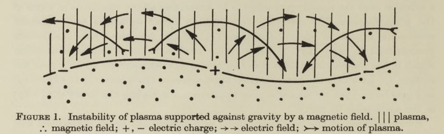
16.2 Plasma supported by magnetic field against gravity

We can start now to consider how magnetic fields change this story by considering cold fluid that is supported from underneath by a magnetic field. Imagine a magnetic field which is decreasing vertically with a density that that is rising vertically.

Assume:

No gas pressure: $p_0 = 0$
Straight magnetic field $\vect {B}_0 = B_0(z)\vect {e}_x$
Gravity $\vect {g} = -g \vect {e}_z$

The equilibrium condition becomes

\frac {d}{dz}\frac {B_0^2(z) }{2\mu _0} = -\rho _0(z) g

The energy variation reduces to

\begin{aligned}2\delta W & = \int dV \left [ \frac {|\vect {Q}|^2}{\mu _0} +\vect {\xi }\cdot \vect {g}\,\nabla \cdot (\rho _0\vect {\xi }) \right ].\end{aligned}

Choose interchange-type perturbations:

\vect {k}\perp \vect {B}_0, \qquad k_\parallel = 0,

so that field lines are exchanged but not bent.

In this case

\vect {Q}_\perp = i k_\parallel B \vect {\xi }_\perp = 0;

the perturbed magnetic field is entirely compressional and parallel to $\vect {B}_0$, and can be minimized by careful choice:

\begin{aligned}\vect {Q} & = \nabla \times \bm {\xi } \times \bm {B}_0\\ & = -\bm {B} \nabla \cdot \bm {\xi }_\perp -\bm {\xi }_\perp \cdot \nabla \bm {B} \\ \left | \bm {Q}^2 \right | & = B_0^2 \left (\nabla \cdot \bm {\xi }_\perp + \bm \xi _\perp \cdot \frac {\nabla B_0}{B_0}\right )^2 \\ \mbox {Choose } & \Rightarrow \quad \nabla \cdot \vect {\xi }_\perp = - \vect {\xi }_\perp \cdot \nabla \ln B_0.\end{aligned}

to mimimize $\delta W$.

Substituting into $\delta W$ gives

\begin{aligned}2\delta W &= \int dV \, \cancel {\left |\vect {Q}^2\right |} + \vect {\xi }\cdot \vect {g} \, \left ( \vect {\xi }_\perp \cdot \nabla \rho _0 + \rho _0 \underbrace {\nabla \cdot \vect {\xi }_\perp }_{ - \vect {\xi }_\perp \cdot \nabla \ln B_0} \right ) \nonumber \\ &= -\int dV \, \rho _0 g \, \xi _z \left ( \vect {\xi }_\perp \cdot \nabla \ln \frac {\rho _0}{B} \right ) \nonumber \\ &= -\int dV \, \rho _0 g \, \frac {d}{dz} \left (\ln \frac {\rho _0}{B_0} \right ) \xi _z^2\end{aligned} \tag{16.37}

\[ \boxed { \text {Magnetic interchange instability if } \frac {d}{dz}\left (\frac {\rho _0}{B_0}\right ) > 0 } \]

Physically: heavy flux tubes above light ones are unstable Kruskal and Schwarzschild (1954).

16.3 Magnetic Buoyancy and Flute-Like Interchange

Now let a horizontal magnetic field help support the atmosphere,

\vect {B}_0=B_0(z)\,\vect {e}_y, \qquad \vect {g}=-g\,\ez ,

where $\vect {e}_y$ is the horizontal field direction. The static equilibrium condition is

\frac {d}{dz}\left (p_0+\frac {B_0^2}{2\mu _0}\right )=-\rho _0 g. \tag{16.39}

We consider flute or interchange perturbations with

k_\parallel =0, \qquad \vect {\xi }=\xi _x\,\vect {e}_x+\xi _z\,\ez , \tag{16.40}

so field lines are exchanged but not bent.

Figure 16.1: Kruskal–Schwarzschild gravitational interchange: plasma supported against gravity by magnetic pressure. The basic question is whether exchanging neighboring flux tubes lowers or raises the potential energy Kruskal and Schwarzschild (1954).

Field perturbation for interchange modes. Recall the linear perturbation of the magnetic field from Eq. (13.4),

\vect {Q} \equiv \B _1 = \curl (\vect {\xi }\times \B _0) = \cancel {(\B \cdot \grad )\vect {\xi }_\perp } - (\vect {\xi }_\perp \cdot \grad )\B - \B \,\divergence \vect {\xi }_\perp

reduces for $k_\parallel =0$ to a purely parallel perturbation,

\vect {Q} = -B_0\left (\divergence \vect {\xi }+\xi _z\frac {d\ln B_0}{dz}\right )\vect {e}_y. \tag{16.42}

such that the field lines remain straight. The equilibrium current is

\vect {J}_0 = \frac {\curl \vect {B}_0}{\mu _0} = -\frac {1}{\mu _0}\frac {dB_0}{dz}\,\vect {e}_x. \tag{16.43}

Energy principle for flute modes. The ideal-MHD potential energy including gravity is

2\delta W = \int dV\, \left [ \frac {|\vect {Q}|^2}{\mu _0} +\gamma p_0(\divergence \vect {\xi })^2 +(\vect {\xi }\cdot \grad p_0)(\divergence \vect {\xi }) -\vect {\xi }\cdot (\vect {J}_0\times \vect {Q}) +(\vect {\xi }\cdot \vect {g})\bigl (\vect {\xi }\cdot \grad \rho _0+\rho _0\divergence \vect {\xi }\bigr ) \right ]. \tag{16.44}

Substitute Eqs. (16.42) and (16.43). First,

\begin{aligned}\frac {|\vect {Q}|^2}{\mu _0} &= \frac {B_0^2}{\mu _0} \left (\divergence \vect {\xi }+\xi _z\frac {d\ln B_0}{dz}\right )^2, \nonumber \\ -\vect {\xi }\cdot (\vect {J}_0\times \vect {Q}) &= -\xi _z\frac {d}{dz}\left (\frac {B_0^2}{2\mu _0}\right ) \left (\divergence \vect {\xi }+\xi _z\frac {d\ln B_0}{dz}\right ).\end{aligned}

Therefore

\begin{aligned}2\delta W &= \int dV\, \Biggl [ \frac {B_0^2}{\mu _0} \left (\divergence \vect {\xi }+\xi _z\frac {d\ln B_0}{dz}\right )^2 +\gamma p_0(\divergence \vect {\xi })^2 +\xi _z\frac {dp_0}{dz}\,\divergence \vect {\xi } \nonumber \\ &\hspace {7em} -\xi _z\frac {d}{dz}\left (\frac {B_0^2}{2\mu _0}\right ) \left (\divergence \vect {\xi }+\xi _z\frac {d\ln B_0}{dz}\right ) -g\xi _z\left (\xi _z\frac {d\rho _0}{dz}+\rho _0\divergence \vect {\xi }\right ) \Biggr ].\end{aligned} \tag{16.46}

Now expand the magnetic square:

\begin{aligned}\frac {B_0^2}{\mu _0} \left (\divergence \vect {\xi }+\xi _z\frac {d\ln B_0}{dz}\right )^2 &= \frac {B_0^2}{\mu _0}(\divergence \vect {\xi })^2 +2\frac {B_0}{\mu _0}\frac {dB_0}{dz}\,\xi _z\divergence \vect {\xi } +\frac {1}{\mu _0}\left (\frac {dB_0}{dz}\right )^2\xi _z^2.\end{aligned}

The current term subtracts

\frac {B_0}{\mu _0}\frac {dB_0}{dz}\,\xi _z\divergence \vect {\xi } + \frac {1}{\mu _0}\left (\frac {dB_0}{dz}\right )^2\xi _z^2,

so one copy of the mixed term remains and the $\xi _z^2$ magnetic term cancels entirely. Hence

\begin{aligned}2\delta W &= \int dV\, \Biggl [ \left (\gamma p_0+\frac {B_0^2}{\mu _0}\right )(\divergence \vect {\xi })^2 +\left (\frac {dp_0}{dz}+\frac {B_0}{\mu _0}\frac {dB_0}{dz}-\rho _0 g\right )\xi _z\divergence \vect {\xi } -g\frac {d\rho _0}{dz}\,\xi _z^2 \Biggr ].\end{aligned}

Using equilibrium, Eq. (16.39), the mixed term becomes $-2\rho _0 g\,\xi _z\divergence \vect {\xi }$, and therefore

2\delta W = \int dV\, \Biggl [ \left (\gamma p_0+\frac {B_0^2}{\mu _0}\right )(\divergence \vect {\xi })^2 -2\rho _0 g\,\xi _z\divergence \vect {\xi } -g\frac {d\rho _0}{dz}\,\xi _z^2 \Biggr ]. \tag{16.50}

Define

c_s^2=\frac {\gamma p_0}{\rho _0}, \qquad v_A^2=\frac {B_0^2}{\mu _0\rho _0}.

Then Eq. (16.50) becomes

\begin{aligned}2\delta W &= \int dV\, \Biggl [ \rho _0(c_s^2+v_A^2)(\divergence \vect {\xi })^2 -2\rho _0 g\,\xi _z\divergence \vect {\xi } -g\frac {d\rho _0}{dz}\,\xi _z^2 \Biggr ].\end{aligned}

Complete the square once more:

\begin{aligned}2\delta W &= \int dV\, \Biggl [ \rho _0(c_s^2+v_A^2) \left (\divergence \vect {\xi }-\frac {g}{c_s^2+v_A^2}\xi _z\right )^2 +\left (-g\frac {d\rho _0}{dz}-\frac {\rho _0 g^2}{c_s^2+v_A^2}\right )\xi _z^2 \Biggr ].\end{aligned} \tag{16.53}

The coefficient of $\xi _z^2$ can be rewritten as

\begin{aligned}-g\frac {d\rho _0}{dz}-\frac {\rho _0 g^2}{c_s^2+v_A^2} &= \frac {g}{c_s^2+v_A^2} \left [ -(c_s^2+v_A^2)\frac {d\rho _0}{dz} +\frac {dp_0}{dz} +\frac {B_0}{\mu _0}\frac {dB_0}{dz} \right ] \nonumber \\ &= \frac {g\rho _0}{c_s^2+v_A^2} \left [ v_A^2\frac {d}{dz}\ln \!\left (\frac {B_0}{\rho _0}\right ) +\frac {c_s^2}{g}N^2 \right ].\end{aligned}

Thus

2\delta W = \int dV\, \rho _0 \left [ (c_s^2+v_A^2) \left (\divergence \vect {\xi }-\frac {g}{c_s^2+v_A^2}\xi _z\right )^2 +N_M^2\xi _z^2 \right ], \tag{16.55}

Now

\mbox {Choose } \qquad \divergence \vect {\xi }-\frac {g}{c_s^2+v_A^2}\xi _z \Rightarrow \quad \nabla \cdot \vect {\xi }_\perp = - \vect {\xi }_\perp \cdot \nabla \ln B_0.

to minimize compression so that

\boxed { N_M^2 \equiv \frac {g}{c_s^2+v_A^2} \left [ v_A^2\frac {d}{dz}\ln \!\left (\frac {B_0}{\rho _0}\right ) +\frac {c_s^2}{g}N^2 \right ]. } \tag{16.57}

This is the magnetic analogue of the Brunt–Väisälä frequency for flute modes. Stability requires $N_M^2>0$.

Cold-plasma limit. If $p_0\to 0$, then $c_s^2\to 0$ and Eq. (16.57) reduces to

N_M^2 \longrightarrow g\frac {d}{dz}\ln \!\left (\frac {B_0}{\rho _0}\right ).

Therefore a cold plasma supported by magnetic pressure is unstable when

\boxed { \frac {d}{dz}\left (\frac {\rho _0}{B_0}\right )>0. } \tag{16.59}

This is the Kruskal–Schwarzschild interchange criterion: the unstable ordering is the magnetic analogue of putting heavy fluid on top of light fluid. Here the relevant quantity is not density alone but mass per unit flux.

Finite-$\beta $ interpretation from a thin flux tube. Equation (16.57) can be understood directly from flux freezing. Along a moving element, the induction and continuity equations imply the familiar frozen-in relation from Eq. (2.7),

\frac {B}{\rho }=\text {const along a fluid element}. \tag{16.60}

Hence

\frac {B_1}{B_0}=\frac {\rho _1}{\rho _0}. \tag{16.61}

From this, one can derive that

\begin{aligned}\delta \rho & = \rho _0 \frac {\delta B^2/2 }{B_0^2} \\ & \frac {1}{v_A^2} \delta (B^2/2 \mu _0)\end{aligned} \tag{16.63}

Magnetic pressure as a $\gamma =2$ fluid. Equation (16.60) has an important thermodynamic reading. For these flute/interchange motions the field is simply carried with the mass, so along a moving element one has $B\propto \rho $. Therefore the magnetic pressure

p_B\equiv \frac {B^2}{2\mu _0} \propto \rho ^2, \qquad \Longrightarrow \qquad \frac {p_B}{\rho ^2}=\text {const along a fluid element}. \tag{16.64}

In that restricted sense the magnetic field behaves like a compressive medium with an effective adiabatic index $\gamma _B=2$. This is stiffer than a monatomic gas, for which $p\propto \rho ^{5/3}$: under compression the magnetic pressure rises faster, and under expansion it falls faster. The corresponding incremental stiffness is

\left .\frac {dp_B}{d\rho }\right |_{\text {frozen-flux}} = \frac {B^2}{\mu _0\rho } = v_A^2,

which is exactly why Eq. (16.63) contains the combination $c_s^2+v_A^2$. In other words, for these $k_\parallel =0$ buoyancy motions the field contributes to the restoring force like an extra pressure law with $\gamma =2$. One should not push the analogy too far: the field is not a true scalar gas because in general it also carries anisotropic tension. But for flute modes, where field lines are exchanged without being bent, this $\gamma =2$ picture captures the essential magnetic compressibility. In that sense, the quantity $p_B/\rho ^2$ plays much the same bookkeeping role for the field that $p/\rho ^\gamma $ plays for an adiabatic gas parcel.

Physical picture. For a tube displaced upward by $\xi _z$, pressure balance with the surrounding atmosphere at the new height gives

\begin{aligned}\delta \left ( p + \frac {B^2}{2 \mu _0} \right )_{\rm parcell} & = \xi _z\frac {d}{dz}\left (p_0+\frac {B_0^2}{2\mu _0}\right ) \nonumber \\ \left ( \pp {p}{\rho } + \pp {p_B} {\rho } \right ) \rho _1 & = -\rho _0 g\,\xi _z \nonumber \\ (c_s^2 + v_A^2) \rho _1 & = -\rho _0 g\,\xi _z \nonumber\end{aligned}

The surrounding atmosphere at the new height has density $\rho _0+\xi _z\rho _0'$, so the density contrast is

\Delta \rho = \rho _1-\xi _z\frac {d\rho _0}{dz}.

The vertical equation of motion is therefore

\begin{aligned}\ddot {\xi }_z & = -g\frac {\Delta \rho }{\rho _0} \nonumber \\ & =-\frac {g}{\rho _0} \left ( -\frac {\rho _0 g}{c_s^2+v_A^2}\,\xi _z -\frac {d\rho _0}{dz} \xi _z\right ) \nonumber \\ & =-\frac {g}{\rho _0} \left ( \frac {1}{c_s^2+v_A^2} \left ( \dd {p_0}{z} + \frac {d}{dz} \frac {B^2}{2 \mu _0} \right ) -\frac {d\rho _0}{dz} \right ) \xi _z \nonumber \\ & =- \frac {g}{c_s^2+v_A^2} \left ( \frac {1}{\rho _0} \left ( \dd {p_0}{z} + \frac {d}{dz} \frac {B^2}{2 \mu _0} \right ) - \frac {c_s^2 + v_A^2}{\rho _0} \frac {d\rho _0}{dz} \right ) \xi _z \nonumber \\ & =- \frac {g}{c_s^2+v_A^2} \left ( \frac {1}{\rho _0} \frac {d}{dz} \frac {B^2}{2 \mu _0} + \frac { v_A^2}{\rho _0}\frac {d\rho _0}{dz} + c_s^2 \left ( \frac {1}{\gamma p_0} \dd {p_0}{z} - \frac {1}{\rho _0} \frac {d\rho _0}{dz} \right ) \right ) \xi _z \nonumber \\ & =- \frac {g}{c_s^2+v_A^2} \left ( \frac {1}{\rho _0} \frac {d}{dz} \frac {B^2}{2 \mu _0} - \frac { v_A^2}{\rho _0}\frac {d\rho _0}{dz} + c_s^2 \left ( \frac {1}{\gamma p_0} \dd {p_0}{z} - \frac {1}{\rho _0} \frac {d\rho _0}{dz} \right ) \right ) \xi _z \nonumber \\ & =- \frac {g}{c_s^2+v_A^2} \left ( v_A^2 \frac {d}{dz} \ln \frac {B}{\rho _0} + c_s^2 N^2 \right ) \xi _z \nonumber \\ &= -N_M^2\xi _z,\end{aligned} \tag{16.67}

and one recovers exactly Eq. (16.57). The first piece of $N_M^2$ measures how magnetic support changes with height; the second is the ordinary Schwarzschild buoyancy term.

Caution

Flute versus Parker. For $k_\parallel =0$, field lines are exchanged but not bent, and the problem is controlled by the magnetic buoyancy frequency $N_M$. The Parker problem is qualitatively different because one allows a small but finite $k_\parallel $: field lines bend, plasma drains along them, and a new competition appears between buoyancy and line tension. That is the gravitational ancestor of ballooning theory.

16.4 The Parker Instability

Magnetic buoyancy plays a central role in connecting the deep-seated solar dynamo to the magnetic structures observed at the solar surface. In dynamo theory, as already discussed in Lecture 8, differential rotation stretches poloidal field into strong toroidal field in the solar interior through the $\Omega $–effect. Once the toroidal field becomes sufficiently strong, magnetic pressure partially replaces gas pressure within the field concentration, reducing the plasma density relative to the surrounding medium.

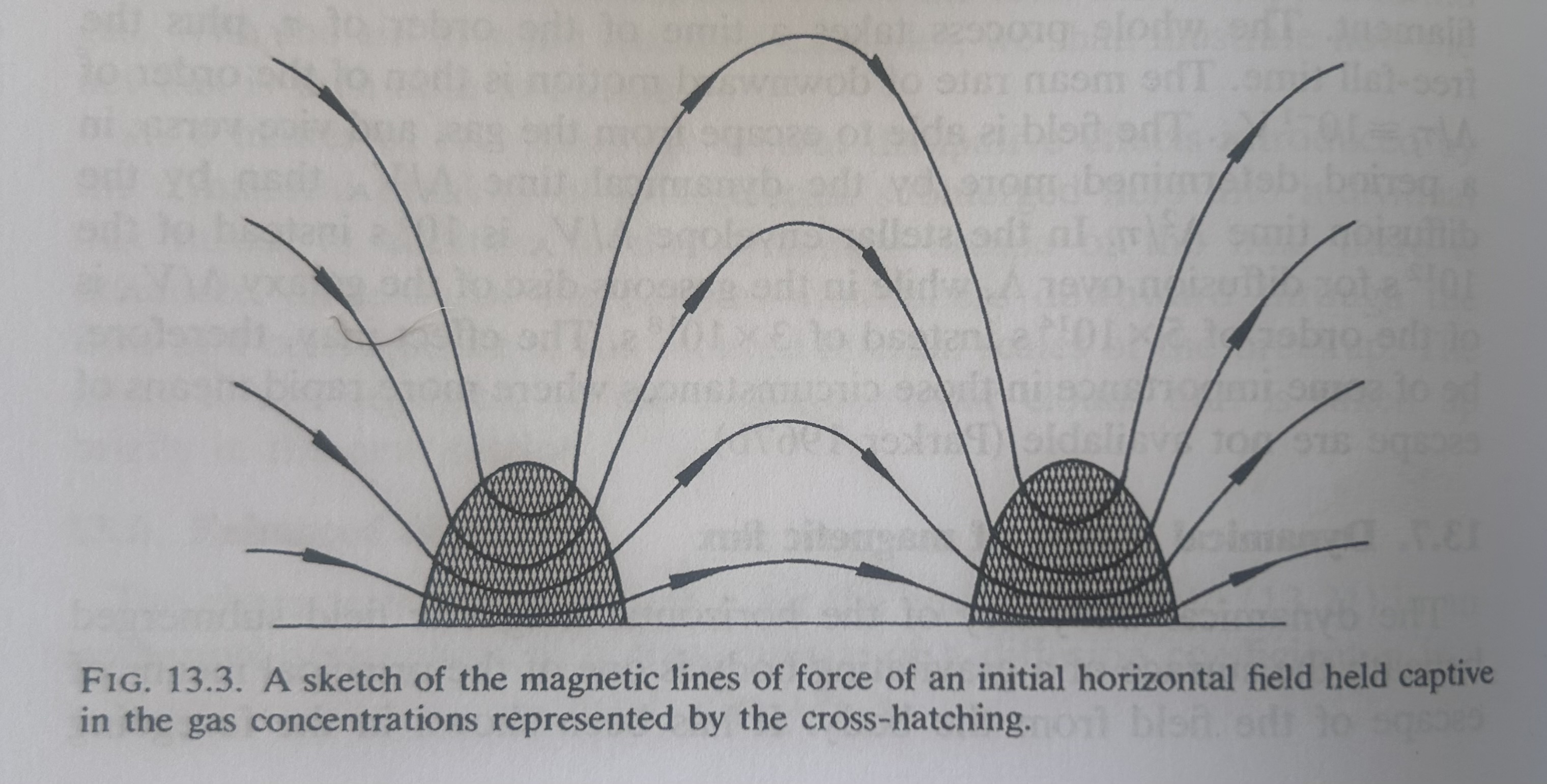
In a gravitationally stratified atmosphere this configuration becomes buoyant. As first described by Parker, undular perturbations of a horizontal magnetic field allow plasma to drain along the field from the tops of rising arches into adjacent troughs. This drainage enhances the density deficit at the crest of the loop, driving the exponential growth of buoyant magnetic structures. These rising loops are widely believed to be the progenitors of sunspot pairs and active regions emerging through the photosphere.

Magnetic buoyancy therefore provides the physical mechanism that transports magnetic flux from the dynamo region to the solar surface. The classical theoretical framework originates in Parker’s early work on magnetic buoyancy and solar dynamos Parker (1955b, 1966, 1979), together with the general stability theory of stratified magnetized plasmas developed by Newcomb and Chandrasekhar Newcomb (1961); Chandrasekhar (1961). Modern numerical work on thin flux tubes rising through the solar convection zone has shown that buoyant loops with strengths of order $10^4$–$10^5$ G reproduce many observed properties of active regions, including emergence latitudes and systematic tilts consistent with Joy’s law Fan et al. (1993); Caligari et al. (1995). Despite this success, several key questions remain unresolved. It is still debated where the toroidal field is generated and stored (tachocline versus distributed convection-zone dynamos), how strong the magnetic field must be to survive turbulent shredding during buoyant rise, and how rotation and convection combine with magnetic tension to produce the observed properties of emerging sunspot pairs. Magnetic buoyancy thus remains a crucial nonlinear link between solar dynamo theory and the surface manifestations of solar activity.

The additional degree of freedom. The energy-principle argument becomes an undular calculation when a long but finite wavelength is admitted along the magnetic field Kulsrud (2005). The perpendicular displacement still raises or lowers a slender flux tube, but the plasma can now slip along that tube. The total compression is therefore \[ \nabla \cdot \vect {\xi } = \nabla \cdot \vect {\xi }_\perp +ik_\parallel \xi _\parallel . \] The new terms have opposite roles. Field-line bending contributes the positive energy $k_\parallel ^2B_0^2\xi _\perp ^2/\muo $, whereas parallel motion couples to buoyancy through \[ i(\vect {g}\cdot \vect {\xi }_\perp )\rho _0k_\parallel \xi _\parallel =-ik_\parallel \xi _zg\rho _0\xi _\parallel . \] The latter contribution can be negative because the relative phase of $\xi _\parallel $ and $\xi _z$ is free to adjust. This phase freedom is the variational expression of plasma draining from the crest of a rising field line.

The low-pressure calculation makes this competition explicit.

Low-pressure limit. For $c_s^2=0$, or equivalently $\beta =c_s^2/v_A^2\ll 1$, the magnetic-compression energy is minimized by the condition already used in Eq. (16.37):

\begin{aligned}\nabla \cdot \vect {\xi }_\perp & = - \vect {\xi }_\perp \cdot \nabla \ln B \mbox { or equivalently}\\ i k_\perp \xi _\perp & = -\xi _z \frac {d}{dz} \ln B_0 \mbox { that leads directly to } \\ k_\perp ^2 \xi _\perp ^2 & = \frac {g^2}{v_A^4} \xi _z^2.\end{aligned}

Adding field-line bending and the coupling to parallel motion gives

\begin{aligned}2\delta W &= \int dV \, \underbrace {k_\parallel ^2 \frac {B_0^2}{\mu _0} \xi _\perp ^2}_{\rm field\, line \,bending } - \rho _0 g \, \xi _z^2 \left ( \dd {}{z} \ln \frac {\rho _0}{B_0} \right ) + \underbrace {2 i \rho _0 g\xi _z k_\parallel \xi _\parallel }_{\rm parallel \, streaming} .\end{aligned}

The factor of two comes from $\vect {\xi }_\parallel \cdot \vect {J}_0\times \vect {Q}_\perp =i\rho _0g\xi _zk_\parallel \xi _\parallel $. The competition is transparent if $\xi _z$ is chosen real and $\xi _\parallel =iA \xi _z$, placing the parallel motion $90^\circ $ out of phase with the vertical displacement. The energy principle then becomes

\begin{aligned}2\delta W &= \int dV \, \rho _0 g \left [ \frac {k_\parallel ^2}{k_\perp ^2} \frac {g}{v_A^2} - \, \left ( \dd {}{z} \ln \frac {\rho _0}{B_0} \right ) - 2 A k_\parallel \right ] \xi _z^2\end{aligned}

and for instability

k_\parallel A = k_\parallel \frac {|\xi _\parallel |}{|\xi _z|} > \frac {k_\parallel ^2}{k_\perp ^2} \frac {g}{v_A^2} - \, \left ( \dd {}{z} \ln \frac {\rho _0}{B_0} \right )

For sufficiently small $k_\parallel $, the line-bending term is weak while parallel drainage remains available. The undular mode can therefore be unstable even when $d\ln (\rho _0/B_0)/dz<0$, a profile that would be stable to a purely interchange perturbation.

The solar tachocline. The base of the solar convection zone (near the tachocline at $r \approx 0.71R_\odot $) is a strongly high–$\beta $ plasma, meaning that gas pressure greatly exceeds magnetic pressure. Typical thermodynamic conditions there are $p \sim 10^{13}$–$10^{14}\,\mathrm {Pa}$ and $\rho \sim 0.2\,\mathrm {kg\,m^{-3}}$. Even if the solar dynamo produces strong toroidal magnetic fields of order $1$–$10\,\mathrm {T}$, the plasma beta

\beta = \frac {2\mu _0 p}{B^2} = \frac {c_s^2}{v_A^2}

remains extremely large, typically \[ \beta \sim 10^{5} - 10^{7}. \]

Thus the equilibrium structure of the plasma is primarily determined by gas pressure and gravity, while magnetic fields act as a relatively small perturbation embedded in the fluid.
If entropy decreases with height, the Schwarzschild criterion predicts convective overturning. The resulting convection drives the stratification toward marginality, consistent with helioseismology and standard solar models.
Magnetic forces play only a weak role in the background equilibrium, and self-organized convection maintains $N^2\approx 0$.
Near the interface between the turbulent convection zone and the radiative interior—the tachocline—differential rotation continually winds poloidal field into toroidal field through the $\Omega $-effect described in Lecture 8.

This high–$\beta $ regime is precisely the one assumed in Parker’s theory of magnetic buoyancy Parker (1955a, 1979), where a modest reduction in gas pressure inside a magnetic flux tube produces a density deficit that allows the tube to rise through the stratified convection zone. Parker’s question was how a long, thin tube of toroidal magnetic flux, wound up by differential rotation near the tachocline, could detach, rise through the turbulent convection zone without being shredded, emerge as a sunspot pair, and contribute to the $\alpha $-effect that closes the dynamo loop.

High-$\beta $ undular modes. At high $\beta $, the displacement is fully three-dimensional and the pressure energy depends on the total compression rather than only on perpendicular compression. The additional terms separate into parallel compression and the coupling between the equilibrium pressure gradient and parallel displacement:

\begin{aligned}2\delta W &= \int dV \, k_\parallel ^2 \frac {B_0^2}{\mu _0} \xi _\perp ^2 + \frac {g\rho _0}{ c_s^2 + v_A^2} \left ( v_A^2 \dd {}{z} \ln \frac {B_0}{\rho _0} + \frac {c_s^2}{g} N^2 \right ) \xi _z^2 + 2 i \rho _0 g\xi _z k_\parallel \xi _\parallel \\ & + \gamma p_0 \left [ (\nabla \cdot \bm {\xi })^2 - (\nabla \cdot \bm {\xi }_\perp )^2\right ] + (\bm {\xi }_\perp \cdot \nabla p_0)(\nabla \cdot \bm {\xi }_\parallel )\end{aligned}

The identities needed to collect these terms are

\begin{aligned}(\nabla \cdot \bm {\xi })^2 - (\nabla \cdot \bm {\xi }_\perp )^2 & = i k_\parallel \xi _\parallel \nabla \cdot \vect {\xi }_\perp ^* - i k_\parallel \xi _\parallel ^* \nabla \cdot \vect {\xi }_\perp + k_\parallel ^2 \xi _\parallel ^2 \\ \nabla \cdot \vect {\xi }_\parallel & = i k_\parallel \xi _\parallel \\ \nabla \cdot \vect {\xi }_\perp = \xi _z \frac {g}{( c_s^2 + v_A^2 )} & \rightarrow \xi _\perp ^2 = \frac {g^2}{k_\perp ^2 (c_s^2 + v_A^2)^2} \xi _z^2\end{aligned}

With these pieces

\begin{aligned}2\delta W &= \int dV \, k_\parallel ^2 \frac {B_0^2}{\mu _0} \xi _\perp ^2 + \frac {g\rho _0}{ c_s^2 + v_A^2} \left ( v_A^2 \dd {}{z} \ln \frac {B_0}{\rho _0} + \frac {c_s^2}{g} N^2 \right ) \xi _z^2 \nonumber \\ + 2 i \rho _0 g\xi _z k_\parallel \xi _\parallel \nonumber \\ & + \gamma p_0 \left ( i k_\parallel (\xi _\parallel \xi _z^* -\xi _\parallel ^* \xi _z) \frac {g}{( c_s^2 + v_A^2 )} + k_\parallel ^2 \xi _\parallel ^2\right ) + \xi _z \dd {p_0}{z} i k_\parallel \xi _\parallel \nonumber \\ &= \int dV \, k_\parallel ^2 \frac {B_0^2}{\mu _0} \xi _\perp ^2 + \gamma p_0 k_\parallel ^2 \xi _\parallel ^2 + \frac {g\rho _0}{ c_s^2 + v_A^2} \left ( v_A^2 \dd {}{z} \ln \frac {B_0}{\rho _0} + \frac {c_s^2}{g} N^2 \right ) \xi _z^2 \nonumber \\ & + i k_\parallel \left ( \left ( 2 \rho _0 g + \dd {p_0}{z} \right ) \xi _z \xi _\parallel + \rho _0 g \frac {c_s^2}{ c_s^2 + v_A^2 } (\xi _\parallel \xi _z^* -\xi _\parallel ^* \xi _z) \right ) \nonumber \\ &= \int dV \, \rho _0 k_\parallel ^2 (v_A^2 \xi _\perp ^2 + c_s^2 \xi _\parallel ^2) + \frac {g\rho _0}{ c_s^2 + v_A^2} \left ( v_A^2 \dd {}{z} \ln \frac {B_0}{\rho _0} + \frac {c_s^2}{g} N^2 \right ) \xi _z^2 \nonumber \\ & + i k_\parallel \left ( \left ( 2 \rho _0 g + \dd {p_0}{z} \right ) \xi _z \xi _\parallel + \rho _0 g \frac {c_s^2}{ c_s^2 + v_A^2 } (\xi _\parallel \xi _z^* -\xi _\parallel ^* \xi _z) \right ) \nonumber\end{aligned}

The pressure term changes the quantitative stability boundary, but the phase relation remains decisive: the last line can be negative when $\xi _\parallel $ and $\xi _z$ acquire the appropriate relative phase. Unlike the low-$\beta $ limit, however, pressure now resists drainage along the field.

Newcomb carried the minimization through and showed that the undular mode is unstable when Newcomb (1961)

- \frac {d\rho }{dz}<\frac {\rho ^2 g}{\gamma p}

or equivalently

\frac {B}{\mu _0 } \frac {d B}{dz} < - \frac {\gamma p N^2}{g}

For $N^2\approx 0$, the condition reduces to $dB/dz<0$: a horizontal field that weakens with height is vulnerable to a sufficiently long-wavelength undular displacement. The variational criterion determines whether the mode exists; the flux-tube picture supplies the corresponding physical image of rising crests and draining plasma.

Why long-wavelength motion along the field matters. In a flute mode the displacement has $k_\parallel =0$, so there is no field-line bending energy and no opportunity for mass to drain from the crest of a rising perturbation to neighboring troughs. Once we allow a small but finite $k_\parallel $, two new effects appear simultaneously:

1.: magnetic tension adds a stabilizing term of order $\rho _0 v_A^2 k_\parallel ^2|\xi _z|^2$,
2.: parallel motion lets plasma slip along the field, which can lighten the crest of a rising arch and thereby increase the buoyancy drive.

The Parker instability is the statement that for sufficiently long parallel wavelength, the second effect can beat the first.

Figure 16.2: The Parker or undular instability: a horizontal field bows upward, plasma drains from the crest to the valleys, and the crest becomes lighter still. This is the prototype of a ballooning mode in a gravitationally stratified atmosphere. The mode is localized across the field but long along it, so the crest can drain mass into the neighboring valleys.

A clean long-wavelength estimate. Take a horizontal flux tube whose crest is displaced upward by $\xi _z$. Let

H_B^{-1}\equiv -\frac {d\ln \rho _0}{dz}

be the density scale height of the background atmosphere and

H_p\equiv \frac {c_s^2}{g}

the gas-pressure scale height along the field line. In a long-wavelength undular mode, pressure equilibrates rapidly along the field, so the crest density of the displaced tube follows the gas-pressure law rather than the full magnetostatic law. To first order,

\rho _{\rm crest}\simeq \rho _0\left (1-\frac {\xi _z}{H_p}\right ), \qquad \rho _{\rm ext}\simeq \rho _0\left (1-\frac {\xi _z}{H_B}\right ).

Thus

\Delta \rho \equiv \rho _{\rm crest}-\rho _{\rm ext} = -\rho _0\left (\frac {1}{H_p}-\frac {1}{H_B}\right )\xi _z. \tag{16.85}

The buoyancy force density is $-g\Delta \rho $, while field-line bending supplies a restoring force density $-\rho _0 v_A^2k_\parallel ^2\xi _z$. Therefore

\ddot {\xi }_z = \left [ g\left (\frac {1}{H_p}-\frac {1}{H_B}\right )-v_A^2k_\parallel ^2 \right ]\xi _z. \tag{16.86}

The long-wavelength undular mode is unstable when

\boxed { k_\parallel ^2 < \frac {g}{v_A^2}\left (\frac {1}{H_p}-\frac {1}{H_B}\right ). } \tag{16.87}

Equivalently, only sufficiently long parallel wavelengths are unstable:

\lambda _\parallel > \lambda _c \equiv \frac {2\pi v_A}{\sqrt {g(H_p^{-1}-H_B^{-1})}}. \tag{16.88}

This estimate is deliberately simple, but it captures the central Parker idea: magnetic support changes the background scale height, while parallel drainage makes the crest obey the gas-pressure scale height instead.

Connection with the exact energy-principle criterion. The full Newcomb treatment is more careful than the estimate above, but it leads to the same lesson: long parallel wavelength and parallel drainage make the configuration easier to destabilize than a purely flute perturbation Newcomb (1961). In the high-$\beta $ limit the instability condition can be written in the compact form

\boxed { \frac {B_0}{\mu _0}\frac {dB_0}{dz} < -\frac {\gamma p_0}{g}N^2. } \tag{16.89}

If the atmosphere is close to adiabatic, so that $N^2\approx 0$, this reduces to the simple statement that a horizontal field which decreases with height is Parker unstable provided the parallel wavelength is long enough.

Bridge to magnetic curvature. In a torus, true gravity is no longer essential. Magnetic curvature and pressure gradient combine to produce an effective buoyancy drive. In that sense, bad curvature in a tokamak or stellarator plays the role that gravity played here, while long parallel wavelength and localization along a field line produce the ballooning structure. The gravitational interchange problem is therefore the clean prototype for magnetic interchange and ballooning theory: first learn the buoyancy physics here, then replace gravity by curvature in the confinement geometry.

Takeaways

The Brunt–Väisälä frequency $N$ measures whether a stratified atmosphere restores or amplifies a vertical displacement.

In a magnetized atmosphere with $k_\parallel =0$, the relevant restoring quantity is the magnetic buoyancy frequency $N_M$, Eq. (16.57).

The cold-plasma interchange criterion depends on $\rho /B$, not on $\rho $ alone: mass per unit magnetic flux is the quantity that gets exchanged.

Allowing finite $k_\parallel $ changes the problem qualitatively. Parallel drainage can overcome line tension and produce Parker’s undular instability, the gravitational prototype of ballooning.

Bibliography

Lord Rayleigh. On convection currents in a horizontal layer of fluid, when the higher temperature is on the under side. Philosophical Magazine, 32:529–546, 1916. doi:10.1080/14786441608635602.

K. Schwarzschild. On the equilibrium of the Sun's atmosphere. Nachrichten von der Gesellschaft der Wissenschaften zu Göttingen, pages 41–53, 1906.

V. Väisälä. Über die wirkung der windschwankungen auf die pilotballonaufstiege. Annales Academiae Scientiarum Fennicae, 24:1–41, 1925.

D. Brunt. The period of simple vertical oscillations in the atmosphere. Quarterly Journal of the Royal Meteorological Society, 53:30–32, 1927. doi:10.1002/qj.49705322103.

M. D. Kruskal and M. Schwarzschild. Some instabilities of a completely ionized plasma. Proceedings of the Royal Society of London A, 223:348–360, 1954. doi:10.1098/rspa.1954.0120.

W. A. Newcomb. Convective instability induced by gravity in a plasma with a frozen-in magnetic field. Physics of Fluids, 4:391–396, 1961. doi:10.1063/1.1706342.

Eugene N Parker. The formation of sunspots from the solar toroidal field. The Astrophysical Journal, 121:491, 1955a. doi:10.1086/146010.

E. N. Parker. Hydromagnetic dynamo models. Astrophysical Journal, 122:293–314, 1955b. doi:10.1086/146087.

P. Charbonneau. Dynamo models of the solar cycle. Living Reviews in Solar Physics, 7:3, 2010. doi:10.12942/lrsp-2010-3.

E. N. Parker. Cosmical Magnetic Fields: Their Origin and Activity. Oxford University Press, 1979.

E. N. Parker. The dynamical state of the interstellar gas and field. Astrophysical Journal, 145:811–833, 1966. doi:10.1086/148828.

S. Chandrasekhar. Hydrodynamic and Hydromagnetic Stability. Clarendon Press, Oxford, 1961.

Y. Fan, G. H. Fisher, and E. E. DeLuca. The rise of magnetic flux tubes in the solar convection zone. Astrophysical Journal, 405:390–401, 1993.

P. Caligari, F. Moreno-Insertis, and M. Schüssler. Emerging flux tubes in the solar convection zone. Astrophysical Journal, 441:886–902, 1995. doi:10.1086/175410.

Russell M. Kulsrud. Plasma Physics for Astrophysics. Princeton University Press, Princeton, NJ, 2005. ISBN 9780691120737.

Guided Exercises

Work through the steps in order. The aim is not only to obtain the stated result, but also to check a useful limit and explain the physics in words.

Problem 16.1. Buoyancy as an energy-principle problem

(a): Starting from Eq. (16.24), complete the square and verify Eq. (16.27).
(b): Show that $\delta W\ge 0$ for every admissible displacement if and only if $N^2\ge 0$. Construct a localized trial displacement that lowers the energy when $N^2<0$.
(c): Explain in parcel language why the sign of $N^2$ determines whether a vertical displacement is restored or amplified.

Problem 16.2. Magnetic buoyancy and its limiting cases

(a): Starting from Eq. (16.57), take $v_A\to 0$ and recover the ordinary Brunt–Väisälä frequency.
(b): Take $c_s\to 0$ and recover the Kruskal–Schwarzschild criterion (16.59). Identify the magnetic analogue of the parcel’s compressional stiffness.
(c): Use Eq. (16.86) to derive the critical wavelength (16.88).
(d): Explain why long parallel wavelengths are destabilizing in the Parker problem: distinguish gravitational release from stabilizing field-line bending.