Toroidal Alfvén Eigenmodes | Classic Problems in MHD

← Previous Lecture Contents Next Lecture →

Lecture 26
Toroidal Alfvén Eigenmodes

Overview

Toroidal Alfvén eigenmodes are a classic tokamak problem. They show, in unusually compact form, how geometry changes the spectrum of ideal MHD. In a cylinder the shear-Alfvén branch is a continuum of local field-line resonances. In a torus, neighboring poloidal harmonics couple, the continuum crossing becomes an avoided crossing, and a spectral gap appears where continuum damping is absense. Discrete global mode can then live in that gap. That mathematical fact matters because modes can propagate in this gap that are easily driven by energetic particles and can redistribute or expel them.

Toroidicity is being introduced explicitly for the first time in this part of the notes. In the TAE chapter it appears as a clean nearest-neighbor harmonic coupling in the wave spectrum. The same $R=R_0+r\cos \theta $ geometry will later reappear in toroidal internal-kink refinements, and again in the Mercier and ballooning lectures as curvature and field-line-following couplings in the toroidal energy principle. So this chapter is the spectrum-level introduction to a piece of geometry that will keep returning.

Historical Perspective

The modern TAE story sits on top of several older layers. Alfvén’s original wave is already present in the local ideal-MHD system, but in a torus one must also confront the fact that each magnetic surface has its own parallel wave number and therefore its own local shear-Alfvén frequency. Newcomb’s one-dimensional variational formulation gave the clean language for radial singularities and continua Newcomb (1960). Kieras and Tataronis then gave an especially transparent formulation of the shear-Alfvén continuous spectrum in axisymmetric toroidal equilibria Kieras and Tataronis (1982). The large-aspect-ratio analyses of Cheng, Chen, and Chance made the key observation that the first toroidal correction couples neighboring poloidal harmonics and therefore opens a gap in the Alfvén continuum Cheng et al. (1985); Cheng and Chance (1987). Fu and Van Dam then pointed out the consequence that mattered for fusion: alpha particles and other energetic ions can resonate with a discrete gap mode and drive it unstable Fu and Van Dam (1989). The TFTR observations of beam-driven TAEs turned that point from an elegant theoretical possibility into an experimental reality Wong et al. (1991). The DIII-D beam-driven studies and the early global-mode comparison between theory and experiment made the same lesson concrete in a different experimental setting Heidbrink et al. (1991); Turnbull et al. (1993). Since then the field has broadened into a full spectroscopy of Alfvénic fluctuations—TAEs, EAEs, NAEs, RSAEs, BAEs—with continuum damping, kinetic corrections, and energetic-particle transport all becoming central parts of the subject Berk et al. (1991); Mett and Mahajan (1992); Fasoli et al. (2007); Lauber (2013); Chen and Zonca (2016); Heidbrink (2008); Heidbrink and White (2020).

This lecture is deliberately tied to the earlier large-aspect-ratio Newcomb analysis. It uses the same field-line mismatch

\Delta _m(r)\equiv n-\frac {m}{q(r)}, \tag{25.1}

and the same Newcomb radial displacement $\xi _m(r)$. The aim is to show how the static Newcomb functional becomes a wave functional, how the Alfvén continuum appears as a singular point of the radial equation, and how the first toroidal harmonic opens the TAE gap.

26.1 Physical picture

Start in a cylinder. For a Fourier harmonic

\xi _r(r,\theta ,\varphi ,t)=\xi _m(r)e^{i(m\theta -n\varphi )-i\omega t}, \tag{25.2}

the large-aspect-ratio parallel wave number is

k_{\parallel m}(r) = \frac {1}{R_0}\left (n-\frac {m}{q(r)}\right ) = \frac {\Delta _m(r)}{R_0}. \tag{25.3}

If $q$ varies with radius, then $k_{\parallel m}$ varies from one magnetic surface to the next. The local shear-Alfvén frequency also varies with radius,

\omega _{A,m}(r) = \left |k_{\parallel m}(r)\right |v_A(r) = \left |\Delta _m(r)\right |\frac {v_A(r)}{R_0}, \qquad v_A(r)=\frac {B_0}{\sqrt {\mu _0\rho (r)}}. \tag{25.4}

The cylinder therefore does not give one global shear-Alfvén frequency. It gives a family of local field-line resonances: the shear-Alfvén continuum.

Now add toroidicity. In a large-aspect-ratio tokamak the major radius varies around the poloidal angle,

R(r,\theta )=R_0+r\cos \theta , \qquad \epsilon (r)\equiv \frac {r}{R_0}\ll 1. \tag{25.5}

Because of the magnetic field variation within a flux surface, the $\cos \theta $ couples neighboring poloidal harmonics $m\leftrightarrow m\pm 1$, while preserving the same toroidal mode number $n$. Where two neighboring cylindrical continuum branches would have crossed, toroidicity converts the exact crossing into an avoided crossing. The interval between the split branches is the toroidicity-induced Alfvén gap.

Why that matters. A discrete mode can localize radially in that gap and thereby avoid the strongest ideal continuum resonances over the region where the mode lives. It is not undamped, but the leading continuum singularity has been pushed aside. At that point geometry has done its job; the stability question is handed to energetic particles, kinetic damping, and the detailed global mode structure.

Caution

A gap is not yet a global mode. The local gap is a statement about the spectrum on each surface. A true TAE still needs radial localization and boundary conditions. Only after the coupled radial problem is solved does one obtain a discrete global eigenmode.

26.2 Newcomb Lagrangian for waves

Tutorial

Step 1: start from the same ideal-MHD variational structure. For ideal MHD linearized about a static equilibrium,
$\rho _0\,\partial _t^2\boldsymbol {\xi } = \mathcal {F}(\boldsymbol {\xi }), \tag{25.6}$ where $\mathcal {F}$ is the self-adjoint linearized force operator. With $e^{-i\omega t}$ time dependence, $\mathcal {F}(\hat {\boldsymbol {\xi }})+\omega ^2\rho _0\hat {\boldsymbol {\xi }}=0. \tag{25.7}$ The corresponding Lagrangian is $\mathcal {L}[\hat {\boldsymbol {\xi }}] = \delta W[\hat {\boldsymbol {\xi }}]-\omega ^2K[\hat {\boldsymbol {\xi }}], \tag{25.8}$ where $\delta W = -\frac 12\int d^3x\,\hat {\boldsymbol {\xi }}^{\,*}\cdot \mathcal {F}(\hat {\boldsymbol {\xi }}), \qquad K=\frac 12\int d^3x\,\rho _0|\hat {\boldsymbol {\xi }}|^2. \tag{25.9}$ For an exact eigenfunction, $\omega ^2=\delta W/K$. But the more useful statement here is that $\delta \mathcal {L}=0$ gives the wave equation.

A schematic Alfvén-wave view of the same functional. Before reducing to one dimension, it is helpful to keep in mind the simplest shear-Alfvén balance inside the energy principle:
$\delta W_A \sim \frac 12\int d^3x\,\frac {B^2}{\mu _0}\left |\nabla _\parallel \xi _\perp \right |^2, \qquad \omega ^2K \sim \frac 12\int d^3x\,\rho \,\omega ^2|\xi _\perp |^2 . \tag{25.10}$ For a local Fourier harmonic with $\nabla _\parallel \to i k_\parallel $, this reduces schematically to $\delta W_A \sim \frac 12\int d^3x\,\rho v_A^2 k_\parallel ^2 |\xi _\perp |^2, \qquad \omega ^2K \sim \frac 12\int d^3x\,\rho \omega ^2 |\xi _\perp |^2, \tag{25.11}$ so stationarity gives the familiar local relation $\omega ^2 \sim k_\parallel ^2 v_A^2. \tag{25.12}$ In a torus, the key change is that the line-bending coefficient is not uniform around the surface. The factor $B^2/B_0^2$ multiplying $|\nabla _\parallel \xi _\perp |^2$ is, at large aspect ratio, $\frac {B^2}{B_0^2} \simeq \frac {R_0^2}{R^2(r,\theta )} = 1-2\epsilon (r)\cos \theta +O(\epsilon ^2). \tag{25.13}$ That $\cos \theta $ variation is the seed of toroidal coupling. After Fourier projection it feeds directly into the off-diagonal $m\leftrightarrow m\pm 1$ terms, while the surface-averaged part populates the diagonal $f_m$ and $g_m$ coefficients.

Step 2: separate the static Newcomb coefficients from inertia. The coefficients in the Rosenbluth–Bussac lecture are potential-energy coefficients. In this lecture we should therefore write them first as $f_m^{(W)}$ and $g_m^{(W)}$. The wave coefficients are obtained only after subtracting $\omega ^2K$:
$\mathcal {L}_m(\omega ) = \delta W_m-\omega ^2K_m. \tag{25.14}$ For the radial displacement variable $\xi _m$, the leading cylindrical kinetic energy is not just an edge term. Use the Rosenbluth–Bussac normalization $\mathcal {N}\equiv \frac {2\pi ^2R_0}{\mu _0}. \tag{25.15}$ The small but important point is that an incompressible shear-Alfvén perturbation is not a purely radial displacement. Once $\xi _r=\xi _m$ is specified, incompressibility also fixes the binormal component $\xi _{\eta m}$. On a cylindrical magnetic surface define $\vect {e}_{\eta ,m} = \frac {(m/r)\vect {e}_{\theta } -(n/R_0)\vect {e}_\varphi } {\left (m^2/r^2+n^2/R_0^2\right )^{1/2}}, \qquad k_{\eta m}^2\equiv \frac {m^2}{r^2}+\frac {n^2}{R_0^2} =\frac {M_m}{r^2}, \tag{25.16}$ where $M_m\equiv m^2+\frac {n^2r^2}{R_0^2}. \tag{25.17}$ Thus, to the accuracy needed here, the physical displacement is $\vect {\xi }_m = \xi _m\vect {e}_r+\xi _{\eta m}\vect {e}_{\eta ,m}, \tag{25.18}$ with any remaining transverse component chosen zero because it would add inertia without helping satisfy incompressibility. The divergence constraint is then $\nabla \cdot \vect {\xi }_m = \frac {1}{r}(r\xi _m)' + i k_{\eta m}\xi _{\eta m} =0, \tag{25.19}$ so $\xi _{\eta m} = \frac {i}{\sqrt {M_m}}(r\xi _m)', \qquad |\xi _{\eta m}|^2 = \frac {|(r\xi _m)'|^2}{M_m}. \tag{25.20}$ This is the whole origin of the derivative inertia. The kinetic energy contains both $|\xi _r|^2$ and $|\xi _\eta |^2$: $\frac {\omega ^2K_m}{\mathcal {N}} = \frac 12\int _0^a \mu _0\rho \omega ^2 r \left [ |\xi _m|^2+|\xi _{\eta m}|^2 \right ]dr = \frac 12\int _0^a \mu _0\rho \omega ^2 \left [ r|\xi _m|^2+ \frac {r}{M_m}\left |(r\xi _m)'\right |^2 \right ]dr . \tag{25.21}$ So the derivative term is not a boundary correction and it is not an extra assumption. It is simply the inertia of the binormal displacement required by $\nabla \cdot \boldsymbol {\xi }=0$.
To put (25.21) into Newcomb’s standard $f,g$ form, expand the second term:
$\frac {r}{M_m}|(r\xi _m)'|^2 = \frac {r}{M_m}|r\xi _m'+\xi _m|^2 = \frac {r^3}{M_m}|\xi _m'|^2 + \frac {r}{M_m}|\xi _m|^2 + \frac {r^2}{M_m}\frac {d}{dr}|\xi _m|^2. \tag{25.22}$ The last term is the only part that becomes a surface contribution. With a nonuniform density, $\int _0^a \mu _0\rho \omega ^2 \frac {r^2}{M_m}\frac {d}{dr}|\xi _m|^2dr = \left [ \mu _0\rho \omega ^2\frac {r^2}{M_m}|\xi _m|^2 \right ]_0^a - \int _0^a \mu _0\omega ^2 \left (\frac {\rho r^2}{M_m}\right )' |\xi _m|^2dr . \tag{25.23}$ Therefore the bulk kinetic coefficients are $f_m^{(K)}(r)=\mu _0\rho \frac {r^3}{M_m}, \tag{25.24}$ $g_m^{(K)}(r)= \mu _0 \left [ \rho \left (r+\frac {r}{M_m}\right ) - \left (\frac {\rho r^2}{M_m}\right )' \right ]. \tag{25.25}$ Since the wave functional is $\delta W_m-\omega ^2K_m$, the full Newcomb wave coefficients are $f_m(r,\omega )= f_m^{(W)}(r)-\omega ^2 f_m^{(K)}(r) = f_m^{(W)}(r)-\mu _0\rho \omega ^2\frac {r^3}{M_m}, \tag{25.26}$ $g_m(r,\omega )= g_m^{(W)}(r)-\omega ^2 g_m^{(K)}(r) = g_m^{(W)}(r) - \mu _0\omega ^2 \left [ \rho \left (r+\frac {r}{M_m}\right ) - \left (\frac {\rho r^2}{M_m}\right )' \right ]. \tag{25.27}$ The integration by parts also changes the natural edge term by $\mathcal {B}(\omega ) = \mathcal {B}^{(W)}- \mu _0\rho (a)\omega ^2\frac {a^2}{M_m(a)} \tag{25.28}$ for a free boundary. For the fixed-boundary internal problem this edge term is irrelevant, but the bulk terms in (25.26) and (25.27) remain. This is where the $\rho \omega ^2$ terms enter Newcomb’s $f_m$ and $g_m$.

Step 3: write the one-dimensional wave functional with f and g. After this subtraction has been made, a single harmonic has the form
$\mathcal {L}_m[\xi _m;\omega ] = \frac 12\int _0^a \left [ f_m(r,\omega )|\xi _m'|^2+g_m(r,\omega )|\xi _m|^2 \right ]dr +\frac 12\mathcal {B}(\omega )|\xi _m(a)|^2. \tag{25.29}$

Step 4: vary it once, carefully. Let $\xi _m\rightarrow \xi _m+\varepsilon \chi $. The term linear in $\varepsilon $ is
$\delta \mathcal {L}_m = \Re \left \{ \int _0^a \left [ f_m\xi _m'\chi ^{*\prime }+g_m\xi _m\chi ^* \right ]dr + \mathcal {B}\xi _m(a)\chi ^*(a) \right \}. \tag{25.30}$ Integrating the derivative term by parts, $\int _0^a f_m\xi _m'\chi ^{*\prime }dr = \left [f_m\xi _m'\chi ^*\right ]_0^a - \int _0^a (f_m\xi _m')'\chi ^*dr. \tag{25.31}$ Since $\chi $ is arbitrary in the interior, the Euler–Lagrange equation is $-\frac {d}{dr}\left (f_m\frac {d\xi _m}{dr}\right )+g_m\xi _m=0. \tag{25.32}$ If several harmonics are retained, $\xi (r,\theta ,\varphi )=\sum _m \xi _m(r)e^{i(m\theta -n\varphi )}$, then the same variational step is carried out independently with respect to each $\xi _m^*$. The result is one Euler–Lagrange equation for every retained harmonic, together with the corresponding coupling terms. If the edge is free rather than fixed, the natural boundary condition is $f_m(a)\xi _m'(a)+\mathcal {B}\xi _m(a)=0. \tag{25.33}$ Equivalently, if $\xi _m(a)\neq 0$, $\frac {\xi _m'(a)}{\xi _m(a)}=-\frac {\mathcal {B}(\omega )}{f_m(a)}. \tag{25.34}$ For a fixed perfectly conducting wall located at the boundary flux surface one instead imposes $\xi _m(a)=0$. This is the same distinction between a natural free-edge condition and a prescribed wall displacement that appears in the earlier Newcomb-style chapters.

Step 5: why continua appear in this same equation. The highest-derivative coefficient is $f_m(r,\omega )$. If $f_m$ is smooth and nonzero on $0<r<a$, the radial problem is an ordinary regular eigenvalue problem. If $f_m(r_A,\omega )=0$ at an interior surface, the differential operator is singular. That singular Newcomb solution is the ideal-MHD continuum.

26.3 The leading large-aspect-ratio wave functional

Use the same definitions as Lecture 24:

\Delta _m(r)=n-\frac {m}{q(r)}, \qquad \Sigma _m(r)=n+\frac {m}{q(r)}, \qquad F_m=-\frac {B_0}{R_0}\Delta _m. \tag{25.35}

The leading large-aspect-ratio Newcomb coefficients are

\begin{aligned}f_{m}^{(W)}(r) &= \frac {B_0^2r^3}{m^2R_0^2}\Delta _m^2 \;{\color {blue}\Bigl (\times \frac {R_0^2}{R^2(r,\theta )}\Bigr )}, \\ g_{m}^{(W)}(r) &= \frac {B_0^2r}{m^2R_0^2}(m^2-1)\Delta _m^2 \;{\color {blue}\Bigl (\times \frac {R_0^2}{R^2(r,\theta )}\Bigr )} + \frac {2n^2r^2}{m^2R_0^2}\mu _0p'(r).\end{aligned} \tag{25.36}

The superscript $(W)$ reminds us that these are the potential-energy pieces; the inertial pieces still have to be added before this becomes a wave functional.

Add the inertial term explicitly. With this normalization, the leading kinetic contribution from (25.21) reduces, for $n^2r^2/R_0^2\ll m^2$ and slowly varying density, to

\frac {\omega ^2K_{m}}{\mathcal {N}} = \frac 12\int _0^a \mu _0\rho \omega ^2 \left [ \frac {r^3}{m^2}|\xi _m'|^2 + \frac {m^2-1}{m^2}r|\xi _m|^2 \right ]dr +\hbox {surface term}. \tag{25.38}

The surface term is zero for a fixed boundary and regular axis, but the two bulk terms are not optional. The static potential-energy coefficients are still the same $f_m^{(W)}$ and $g_m^{(W)}$ written above. The blue parenthetical factor is only a reminder at this stage. The one-harmonic coefficients above are obtained after angular projection. To recover the toroidal coupling, one must restore $R_0^2/R^2(r,\theta )=1-2\epsilon \cos \theta +\cdots $ before that projection, so that the $\cos \theta $ term can connect $m$ to $m\pm 1$. The kinetic coefficients from (25.38) are

f_{m}^{(K)}=\mu _0\rho \frac {r^3}{m^2}, \qquad g_{m}^{(K)}=\mu _0\rho \frac {m^2-1}{m^2}r . \tag{25.39}

Subtracting $\omega ^2K_{m}$ from the static leading-order coefficients therefore gives

f_{m}(r,\omega ) = f_{m}^{(W)}-\omega ^2 f_{m}^{(K)} = \frac {r^3}{m^2} \left [ \frac {B_0^2}{R_0^2}\Delta _m^2(r)-\mu _0\rho (r)\omega ^2 \right ], \tag{25.40}

g_{m}(r,\omega ) = g_{m}^{(W)}-\omega ^2 g_{m}^{(K)} = \frac {m^2-1}{m^2}r \left [ \frac {B_0^2}{R_0^2}\Delta _m^2(r)-\mu _0\rho (r)\omega ^2 \right ] + \frac {2n^2r^2}{m^2R_0^2}\mu _0p'(r). \tag{25.41}

Equivalently,

f_{m}=\frac {r^3}{m^2}\mathcal {A}_m, \qquad g_{m}=\frac {m^2-1}{m^2}r\mathcal {A}_m + \frac {2n^2r^2}{m^2R_0^2}\mu _0p', \tag{25.42}

where

\mathcal {A}_m(r,\omega ) \equiv \frac {B_0^2}{R_0^2}\Delta _m^2(r)-\mu _0\rho (r)\omega ^2 = \mu _0\rho (r)\left [\omega _{A,m}^2(r)-\omega ^2\right ]. \tag{25.43}

This is the answer to the apparent mystery in the derivative term: the coefficient multiplying $\xi _m'$ is the line-bending coefficient $r^3B_0^2\Delta _m^2/(m^2R_0^2)$ minus the derivative part of the kinetic metric, $\mu _0\rho \omega ^2r^3/m^2$. Factoring out $r^3/m^2$ leaves $\mathcal {A}_m$. Thus the leading one-harmonic wave functional is

\frac {\mathcal {L}_{m}}{\mathcal {N}} = \frac 12\int _0^a \left [ f_{m}(r,\omega )|\xi _m'|^2+ g_{m}(r,\omega )|\xi _m|^2 \right ]dr . \tag{25.44}

For the elementary TAE derivation below we set the pressure-gradient term aside. That is the low-$\beta $, shear-Alfvén limit.

The useful rule is therefore not “use the static $f$ and $g$ unchanged.” It is

f_m=f_m^{(W)}-\omega ^2 f_m^{(K)}, \qquad g_m=g_m^{(W)}-\omega ^2 g_m^{(K)}. \tag{25.45}

At leading order, this rule is equivalent to replacing

\frac {B_0^2}{R_0^2}\Delta _m^2 \quad \longrightarrow \quad \frac {B_0^2}{R_0^2}\Delta _m^2-\mu _0\rho \omega ^2 \tag{25.46}

inside the leading line-bending pieces of both $f_m$ and $g_m$.

The explicit one-dimensional wave equation. Varying (25.44) gives the Newcomb wave equation

-\frac {d}{dr} \left [ f_{m}(r,\omega )\frac {d\xi _m}{dr} \right ] + g_{m}(r,\omega )\xi _m =0. \tag{25.47}

Using (25.40)–(25.41), this is

-\frac {d}{dr} \left [ \frac {r^3}{m^2}\mathcal {A}_m(r,\omega )\frac {d\xi _m}{dr} \right ] + \left [ \frac {m^2-1}{m^2}r\mathcal {A}_m(r,\omega ) + \frac {2n^2r^2}{m^2R_0^2}\mu _0p'(r) \right ]\xi _m =0. \tag{25.48}

The fixed-boundary version uses regularity at the magnetic axis and $\xi _m(a)=0$ at a perfectly conducting wall. A free edge instead uses the natural boundary condition from (25.33), or equivalently the slope condition $\xi _m'(a)/\xi _m(a)=-\mathcal {B}(\omega )/f_m(a)$ from (25.34).

Where the singularity is. The coefficient of the highest radial derivative vanishes when

\mathcal {A}_m(r_A,\omega )=0, \tag{25.49}

or equivalently

D_m(r_A,\omega ) \equiv \omega ^2-\omega _{A,m}^2(r_A) = \omega ^2-\omega _A^2(r_A)\Delta _m^2(r_A) =0, \tag{25.50}

where $\omega _A(r)=v_A(r)/R_0$. The two signs are useful for different purposes:

\mathcal {A}_m=-\mu _0\rho D_m. \tag{25.51}

Newcomb’s singular-surface language is equivalent to $\mathcal {A}_m=0$, because $\mathcal {A}_m$ multiplies the highest derivative. The continuum language is naturally phrased as $D_m=0$, because $D_m$ is the local oscillator denominator.

Local form of the singular solution. Assume $r_A$ is a simple resonance, so

\mathcal {A}_m(r,\omega ) \simeq \mathcal {A}'_{mA}(r-r_A), \qquad \mathcal {A}'_{mA}\equiv \left .\frac {\partial \mathcal {A}_m}{\partial r}\right |_{r_A}. \tag{25.52}

The leading singular part of (25.48) is then

-\frac {d}{dr} \left [ (r-r_A)\frac {d\xi _m}{dr} \right ] \simeq 0, \tag{25.53}

where smooth nonzero factors have been divided out. Integrating twice,

(r-r_A)\xi _m'=C_1, \qquad \xi _m(r)=C_0+C_1\ln |r-r_A|. \tag{25.54}

Thus the ideal-MHD continuum is not merely the algebraic formula $\omega =\omega _{A,m}(r)$. In the full radial Newcomb problem it is a logarithmic singularity caused by the vanishing of the highest-derivative coefficient.

Caution

Do not confuse two different uses of “resonance.” The rational surface $\Delta _m=0$ is the place where $k_{\parallel m}=0$, so the local shear-Alfvén frequency of that harmonic is zero. A finite-frequency Alfvén continuum resonance satisfies $D_m=0$, i.e. $\omega ^2=\omega _A^2\Delta _m^2$. For a fixed nonzero $\omega $, the resonant surface is generally not the rational surface.

26.4 Toroidal coupling

Where the coupling comes from: project the cosine term explicitly. The off-diagonal coupling is not contained in the already-projected one-harmonic coefficients $f_m$ and $g_m$. It appears only if the poloidal dependence of the toroidal metric is kept before the Fourier projection. The specific factor being expanded is the one multiplying the shear-Alfvén line-bending energy, $B^2/B_0^2$, which in a large-aspect-ratio tokamak with dominantly toroidal field is equivalently $R_0^2/R^2(r,\theta )$. For circular flux surfaces,

\frac {R_0^2}{R^2(r,\theta )} = 1-2\epsilon (r)\cos \theta +O(\epsilon ^2), \qquad \epsilon (r)=\frac {r}{R_0}. \tag{25.55}

With the scalar displacement amplitude written out before the angular integrations, the large-aspect-ratio expansion keeps both the radial-derivative and algebraic pieces explicit. Define \[ \xi (r,\theta ,\varphi ) = e^{-in\varphi }\sum _m \xi _m(r)e^{im\theta }, \qquad S(r,\theta ,\varphi ) \equiv e^{-in\varphi }\sum _m \Delta _m(r)\xi _m(r)e^{im\theta }, \] \[ S_r(r,\theta ,\varphi ) \equiv e^{-in\varphi }\sum _m \Delta _m(r)\frac {r}{m}\frac {d\xi _m}{dr}\,e^{im\theta }, \qquad S_0(r,\theta ,\varphi ) \equiv e^{-in\varphi }\sum _m \sqrt {\frac {m^2-1}{m^2}}\, \Delta _m(r)\xi _m(r)e^{im\theta }, \] \[ \Xi _r(r,\theta ,\varphi ) \equiv e^{-in\varphi }\sum _m \frac {r}{m}\frac {d\xi _m}{dr}\,e^{im\theta }, \qquad \Xi _0(r,\theta ,\varphi ) \equiv e^{-in\varphi }\sum _m \sqrt {\frac {m^2-1}{m^2}}\, \xi _m(r)e^{im\theta }, \] \[ \frac {\mathcal {L}}{\mathcal {N}} = \frac 12\int dr\,\mu _0\rho r \int _0^{2\pi }\frac {d\varphi }{2\pi } \int _0^{2\pi }\frac {d\theta }{2\pi } \Bigg [ \underbrace { \omega _A^2(r)\frac {R_0^2}{R^2(r,\theta )} \Bigl (|S_r|^2+|S_0|^2\Bigr ) }_{\text {toroidally modulated line bending}} - \underbrace { \omega ^2\Bigl (|\Xi _r|^2+|\Xi _0|^2\Bigr ) }_{\text {inertia}} \Bigg ], \] \[ \frac {R_0^2}{R^2(r,\theta )} = \underbrace {1}_{\text {diagonal one-harmonic piece}} \;+\; \underbrace {\bigl (-2\epsilon (r)\cos \theta \bigr )}_{\text {source of }m\leftrightarrow m\pm 1\text { coupling}} \;+\; O(\epsilon ^2). \] Because every coupled sideband carries the same toroidal factor $e^{-in\varphi }$, the $\varphi $ integration is trivial and $n$ remains a good quantum number. One is then left with the $\theta $ integrals that produce the diagonal orthogonality term from the first underbrace and the nearest-neighbor cosine selection rule from the second. The metric factor $R_0^2/R^2(r,\theta )$ multiplies the whole line-bending density $|S|^2$; it may equivalently be written as $|(R_0/R)S|^2$, but not as a term-by-term modification of the Fourier sum itself. After angular projection, the line-bending and inertial pieces recombine harmonic by harmonic into the same diagonal factor $\omega _A^2\Delta _m^2-\omega ^2$, which is exactly the resonant combination appearing in (25.43) and in the full radial wave functional (25.44). The selection rule is just the Fourier identity

\cos \theta \,e^{i(m\theta -n\varphi )} = \frac 12e^{i[(m+1)\theta -n\varphi ]} + \frac 12e^{i[(m-1)\theta -n\varphi ]}. \tag{25.56}

For shorthand after the trivial $\varphi $ integral, write the local line-bending amplitude as

S(r,\theta ) \equiv \sum _m \Delta _m(r)\xi _m(r)e^{im\theta }, \tag{25.57}

where the common factor $e^{-in\varphi }$ has already been suppressed. Likewise,

S_r(r,\theta ) \equiv \sum _m \Delta _m(r)\frac {r}{m}\frac {d\xi _m}{dr}\,e^{im\theta }, \qquad S_0(r,\theta ) \equiv \sum _m \sqrt {\frac {m^2-1}{m^2}}\,\Delta _m(r)\xi _m(r)e^{im\theta }. \tag{25.58}

The diagonal part follows from ordinary orthogonality,

\left \langle e^{i(m-\ell )\theta }\right \rangle _\theta =\delta _{m\ell }, \qquad \left \langle |S|^2\right \rangle _\theta = \sum _m\Delta _m^2|\xi _m|^2. \tag{25.59}

The off-diagonal part follows from the same identity with one factor of $\cos \theta $:

\left \langle \cos \theta \,e^{i(m-\ell )\theta } \right \rangle _\theta = \frac 12\left (\delta _{\ell ,m+1}+\delta _{\ell ,m-1}\right ). \tag{25.60}

Using (25.60) in the derivative and algebraic pieces gives

\left \langle \cos \theta \,|S_r|^2\right \rangle _\theta = \frac 12\sum _m \Delta _m\Delta _{m+1} \frac {r^2}{m(m+1)} \left ( \xi _m^{\prime *}\xi _{m+1}'+\xi _{m+1}^{\prime *}\xi _m' \right ). \tag {28.87a}

The same quantity may equally well be written as

\left \langle \cos \theta \,|S_r|^2\right \rangle _\theta = \frac 12\sum _m \Delta _m\Delta _{m-1} \frac {r^2}{m(m-1)} \left ( \xi _m^{\prime *}\xi _{m-1}'+\xi _{m-1}^{\prime *}\xi _m' \right ), \tag {28.87a$'$}

and

\left \langle \cos \theta \,|S_0|^2\right \rangle _\theta = \frac 12\sum _m \Delta _m\Delta _{m+1} \sqrt {\frac {m^2-1}{m^2}} \sqrt {\frac {(m+1)^2-1}{(m+1)^2}} \left ( \xi _m^*\xi _{m+1}+\xi _{m+1}^*\xi _m \right ). \tag {28.87b}

or equivalently

\left \langle \cos \theta \,|S_0|^2\right \rangle _\theta = \frac 12\sum _m \Delta _m\Delta _{m-1} \sqrt {\frac {m^2-1}{m^2}} \sqrt {\frac {(m-1)^2-1}{(m-1)^2}} \left ( \xi _m^*\xi _{m-1}+\xi _{m-1}^*\xi _m \right ). \tag {28.87b$'$}

The primed forms are identical to the unprimed ones after a dummy-index shift, so the later coupled equations may be written using either neighboring pair $(m,m+1)$ or $(m,m-1)$. These are the crux. The factor $1/2$ comes from the cosine selection rule, while the metric perturbation carries the factor $-2\epsilon \cos \theta $. Their product is $-\epsilon $. The projected wave functional is therefore

\frac {\mathcal {L}}{\mathcal {N}} = \frac 12\int dr\,\mu _0\rho (r)r \left [ \omega _A^2(r) \left \langle \bigl (1-2\epsilon (r)\cos \theta \bigr )\Bigl (|S_r|^2+|S_0|^2\Bigr ) \right \rangle _\theta - \omega ^2 \left \langle |\Xi _r|^2+|\Xi _0|^2 \right \rangle _\theta \right ]. \tag{25.61}

Eigenmode Equations If only the pair $(m,m+1)$ is kept, the derivative part of (25.61) gives the reduced two-harmonic wave functional

\frac {\mathcal {L}_{m,m+1}}{\mathcal {N}} = \frac 12\int dr\, \Bigg [ \frac {r^3}{m^2}\mathcal {A}_m|\xi _m'|^2 + \frac {r^3}{(m+1)^2}\mathcal {A}_{m+1}|\xi _{m+1}'|^2 - \epsilon (r)\frac {r^3B_0^2}{R_0^2} \frac {\Delta _m\Delta _{m+1}}{m(m+1)} \left ( \xi _m^{\prime *}\xi _{m+1}'+\xi _{m+1}^{\prime *}\xi _m' \right ) + \frac {m^2-1}{m^2}r\,\mathcal {A}_m|\xi _m|^2 + \frac {(m+1)^2-1}{(m+1)^2}r\,\mathcal {A}_{m+1}|\xi _{m+1}|^2 \Bigg ]. \tag{25.62}

This is the point where the later off-diagonal derivative block first appears: the term proportional to $\epsilon \,\Delta _m\Delta _{m+1}\,\xi _m^{\prime *}\xi _{m+1}'$ is the ancestor of the off-diagonal entries in $\bm P_\xi $. If one starts instead from the adjacent pair $(m-1,m)$, the reduced functional is

\frac {\mathcal {L}_{m-1,m}}{\mathcal {N}} = \frac 12\int dr\, \Bigg [ \frac {r^3}{(m-1)^2}\mathcal {A}_{m-1}|\xi _{m-1}'|^2 + \frac {r^3}{m^2}\mathcal {A}_{m}|\xi _{m}'|^2 - \epsilon (r)\frac {r^3B_0^2}{R_0^2} \frac {\Delta _{m-1}\Delta _{m}}{(m-1)m} \left ( \xi _{m-1}^{\prime *}\xi _{m}'+\xi _{m}^{\prime *}\xi _{m-1}' \right ) + \frac {(m-1)^2-1}{(m-1)^2}r\,\mathcal {A}_{m-1}|\xi _{m-1}|^2 + \frac {m^2-1}{m^2}r\,\mathcal {A}_{m}|\xi _{m}|^2 \Bigg ]. \tag {28.89$'$}

After the dummy-index relabel $j=m-1$, this becomes precisely $\mathcal {L}_{j,j+1}$. So the recursive use of a single neighboring pair in (25.62) is justified: every adjacent pair is described by the same template, differing only by which local crossing $\Delta _j\simeq \Delta _{j+1}$ is chosen.

Apply Euler-Lagrange: Varying (25.62) with respect to $\xi _m^*$ and $\xi _{m+1}^*$ gives the coupled radial equations

\begin{aligned}-\frac {d}{dr} \left [ \frac {r^3}{m^2}\mathcal {A}_m\xi _m' \right ] \;+\; \frac {d}{dr} \left [ \epsilon (r)\frac {r^3B_0^2}{R_0^2} \frac {\Delta _m\Delta _{m+1}}{m(m+1)}\xi _{m+1}' \right ] \;+\; \frac {m^2-1}{m^2}r\,\mathcal {A}_m\xi _m &=0, \\ -\frac {d}{dr} \left [ \frac {r^3}{(m+1)^2}\mathcal {A}_{m+1}\xi _{m+1}' \right ] \;+\; \frac {d}{dr} \left [ \epsilon (r)\frac {r^3B_0^2}{R_0^2} \frac {\Delta _m\Delta _{m+1}}{m(m+1)}\xi _m' \right ] \;+\; \frac {(m+1)^2-1}{(m+1)^2}r\,\mathcal {A}_{m+1}\xi _{m+1} &=0.\end{aligned} \tag{25.63}

After changing to $x=r/a$, introducing $\lambda =(\omega R_0/v_A)^2$ and $D_\ell =\lambda -\Delta _\ell ^2$, and absorbing overall factors, these become the compact matrix operator written in the next section. Only after freezing the radial coefficients on one surface does one arrive at the local algebraic continuum matrix used to read off the gap.

Thus, in the low-$\beta $ shear-Alfvén limit, the coupled $(m,m+1)$ problem may be written directly for the harmonic-amplitude pair $\mathbf {y}=(\xi _m,\xi _{m+1})^T$ as

\frac {d}{dx} \left [ \bm {P}_{\xi }(x,\lambda )\frac {d\mathbf {y}}{dx} \right ] - \bm {Q}_{\xi }(x,\lambda )\mathbf {y} =0, \tag{25.65}

with

\bm {P}_{\xi }= \begin {pmatrix} x^3D_m & \epsilon \lambda x^4\\[3pt] \epsilon \lambda x^4 & x^3D_{m+1} \end {pmatrix}, \qquad \bm {Q}_{\xi }= \begin {pmatrix} (m^2-1)xD_m & 0\\[3pt] 0 & \left [(m+1)^2-1\right ]xD_{m+1} \end {pmatrix}, \tag{25.66}

where

D_{\ell }(x,\lambda ) \equiv \lambda -\Delta _{\ell }^{2}(x), \qquad \Delta _{\ell }(x)\equiv n-\frac {\ell }{q(x)}, \qquad \lambda \equiv \left (\frac {\omega R_0}{v_A}\right )^2. \tag{25.67}

This is the direct $\xi _r$ version of the Fu–Van Dam radial system. An equivalent two-harmonic formulation was written earlier by Cheng, Chen, and Chance Cheng et al. (1985); Cheng and Chance (1987), and the benchmark shooting version used below was written by Fu and Van Dam Fu and Van Dam (1989). In ideal MHD,

\delta \vect {E} = -\partial _t \boldsymbol {\xi }\times \vect {B}_0 = i\omega \boldsymbol {\xi }\times \vect {B}_0 , \tag{25.68}

so for a dominantly toroidal equilibrium field $\vect {B}_0\simeq B_0\vect {e}_\varphi $,

E_{\theta m}\simeq -\,i\omega B_0\,\xi _m . \tag{25.69}

Thus the Fu–Van Dam equations are simply the same coupled radial problem written in $E_\theta $ rather than $\xi _r$.

The gap is already visible in the highest-order derivatives. To see the local continuum structure, freeze the slowly varying radial coefficients on a chosen surface and focus on the highest-order derivative terms. Then the common $d^2/dx^2$ factor multiplies the matrix $\bm {P}_{\xi }$, so the local singular surfaces are determined by

\det \bm {P}_{\xi }=0. \tag{25.70}

Since

\det \bm {P}_{\xi } = x^6\left [D_mD_{m+1}-\epsilon ^2\lambda ^2x^2\right ], \tag{25.71}

the local continuum condition is

D_mD_{m+1}-\epsilon ^2\lambda ^2x^2=0. \tag{25.72}

After dividing out the harmless common factor $x^3$, this is equivalent to the local two-by-two algebraic system

\begin {pmatrix} \lambda -\Delta _m^2 & \epsilon \lambda x\\[4pt] \epsilon \lambda x & \lambda -\Delta _{m+1}^2 \end {pmatrix} \begin {pmatrix} \xi _m\\ \xi _{m+1} \end {pmatrix} \simeq 0, \tag{25.73}

which is the same avoided-crossing matrix written in dimensionless form.

Keep only the two harmonics that cross. Near the crossing of the $m$ and $m+1$ branches, keep only those two amplitudes. Freezing the coefficients in (25.63)–(25.64) on a single surface reduces the radial system to

\begin {pmatrix} \omega ^2-\omega _A^2\Delta _m^2 & \epsilon \omega _A^2\Delta _m\Delta _{m+1} \\[4pt] \epsilon \omega _A^2\Delta _m\Delta _{m+1} & \omega ^2-\omega _A^2\Delta _{m+1}^2 \end {pmatrix} \begin {pmatrix} \xi _m\\ \xi _{m+1} \end {pmatrix} =0. \tag{25.74}

A nontrivial solution requires

\left (\omega ^2-\omega _A^2\Delta _m^2\right ) \left (\omega ^2-\omega _A^2\Delta _{m+1}^2\right ) - \epsilon ^2\omega _A^4\Delta _m^2\Delta _{m+1}^2 =0. \tag{25.75}

Solving for $\omega ^2$,

\omega _\pm ^2 = \frac {\omega _A^2}{2}\left (\Delta _m^2+\Delta _{m+1}^2\right ) \pm \omega _A^2 \left [ \left (\frac {\Delta _m^2-\Delta _{m+1}^2}{2}\right )^2 + \epsilon ^2\Delta _m^2\Delta _{m+1}^2 \right ]^{1/2}. \tag{25.76}

This is the avoided-crossing formula.

Evaluate it at the crossing. At the uncoupled crossing,

\Delta _m=-\Delta _{m+1}, \qquad |\Delta _m|=|\Delta _{m+1}|=\frac {1}{2q_c}, \tag{25.77}

\omega _0 = \frac {v_A}{2q_cR_0}. \tag{25.78}

Equation (25.76) reduces to

\omega _\pm ^2 = \omega _0^2(1\pm \epsilon _c), \qquad \epsilon _c\equiv \frac {r_c}{R_0}. \tag{25.79}

Therefore

\Delta (\omega ^2)=\omega _+^2-\omega _-^2=2\epsilon _c\omega _0^2, \qquad \Delta \omega \equiv \omega _+-\omega _- \simeq \epsilon _c\omega _0 \quad (\epsilon _c\ll 1). \tag{25.80}

The cylinder would have given an exact crossing. The torus gives a gap whose fractional width is of order inverse aspect ratio.

What is being plotted in the continuum figures. For each surface one first draws the uncoupled cylindrical continua

\omega _{A,m}(r)=\left |\Delta _m(r)\right |\frac {v_A(r)}{R_0}, \qquad \omega _{A,m+1}(r)=\left |\Delta _{m+1}(r)\right |\frac {v_A(r)}{R_0}. \tag{25.81}

Then one retains only the crossing pair $m$ and $m+1$, solves the local two-by-two system (25.74) on that surface, and plots its two eigenvalues $\omega _\pm (r)$ from (25.76). The solid split branches in the figures below are therefore the local toroidal continuum obtained by diagonalizing the coupled continuum matrix on each surface. They are not yet the discrete global TAE eigenfunction; the radial envelope problem still comes afterward.

Takeaways

The leading cylindrical Newcomb equation gives singular continuum surfaces where $D_m=0$. Toroidicity does not remove the continuum everywhere; it couples neighboring singular branches. At the branch crossing, that coupling splits the two local continuum frequencies and opens a gap. A TAE is a global mode that can live in that gap.

26.5 A Fu–Van Dam benchmark

Choose a simple monotone safety-factor profile. Take

q(r)=q_0+(q_a-q_0)\left (\frac {r}{a}\right )^2, \qquad q_0\simeq 1, \qquad q_a\simeq 2. \tag{25.82}

For arithmetic let $q_0=1$ and $q_a=2$. Then

q(r)=1+\frac {r^2}{a^2}. \tag{25.83}

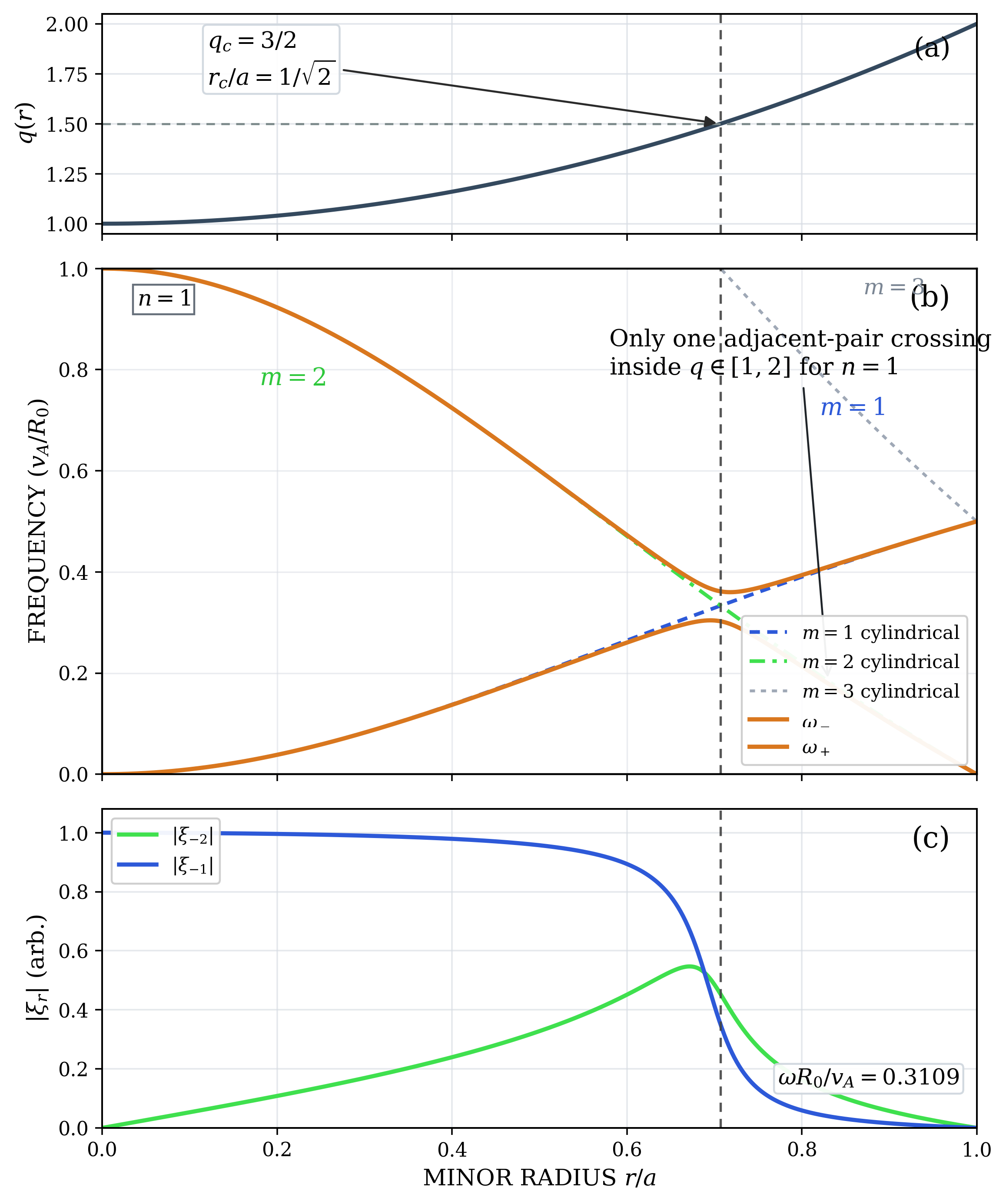
Figure 25.1 is organized around this same benchmark profile. Its top panel shows $q(r)$, the middle panel shows the local $n=1$ continua, and the bottom panel shows the corresponding global eigenmode. A faint $m=3$ cylindrical branch is included in the continuum panel only to show that it remains far above the gap frequency and therefore does not obviously threaten the benchmark mode with nearby continuum damping.

Figure 26.1: Fu–Van Dam benchmark shown as a single three-panel story. (a) The safety-factor profile $q(r)=1+(r/a)^2$, with the TAE crossing at $q_c=3/2$, $r_c/a=1/\sqrt {2}$. (b) The local $n=1$ continua: dashed cylindrical branches for the crossing pair $m=1,2$, the solid toroidally split branches $\omega _\pm (r)$, and a faint $m=3$ cylindrical branch in the upper right that stays far from the gap. The toroidal branches are the local eigenvalues of the coupled two-mode matrix (25.74). (c) The corresponding fixed-wall Fu–Van Dam eigenmode, plotted in the same radial coordinate.

We will be searching for eigen functions that depend on the same $n$ since toroidal axisymmetry conserves the toroidal mode number. The basic TAE pair is therefore the pair

(m,n)=(-2,-1), \qquad (m+1,n)=(-1,-1), \tag{25.84}

At the crossing however the $\Delta _m$, hence $k_\parallel $ are of opposite signs.

Locate the uncoupled crossing. The two cylindrical continuum branches cross when their local Alfvén frequencies are equal,

\omega _A^2\Delta _m^2=\omega _A^2\Delta _{m+1}^2. \tag{25.85}

The crossing relevant to a TAE has opposite parallel wave numbers,

\Delta _m=-\Delta _{m+1}. \tag{25.86}

Using $\Delta _m=n-m/q$,

n-\frac {m}{q_c} = -\left (n-\frac {m+1}{q_c}\right ),

q_c=\frac {m+\tfrac 12}{n}. \tag{25.88}

For $m=-2$ and $n=-1$,

q_c=\frac 32. \tag{25.89}

With (25.83),

\frac {r_c}{a} = \left (\frac {q_c-q_0}{q_a-q_0}\right )^{1/2} = \left (\frac {1.5-1}{2-1}\right )^{1/2} = \frac {1}{\sqrt {2}} \simeq 0.707. \tag{25.90}

At this radius,

\Delta _{-2}(r_c)=-1+\frac {2}{1.5}=+\frac 13, \qquad \Delta _{-1}(r_c)=-1+\frac {1}{1.5}=-\frac 13. \tag{25.91}

Thus both branches satisfy the same continuum-resonance condition at the same radius when

\omega _0 = \omega _A(r_c)|\Delta _{-2}(r_c)| = \omega _A(r_c)|\Delta _{-1}(r_c)| = \frac {v_A(r_c)}{3R_0}. \tag{25.92}

This is the surface where toroidicity will open the gap.

The rational surfaces are nearby but different. For the same profile,

\Delta _{-2}=0 \quad \Longleftrightarrow \quad q=2 \quad \Longrightarrow \quad \frac {r}{a}=1, \tag{25.93}

and

\Delta _{-1}=0 \quad \Longleftrightarrow \quad q=1 \quad \Longrightarrow \quad \frac {r}{a}=0. \tag{25.94}

Those are the zero-frequency continuum points. The TAE crossing at $r_c/a\simeq 0.707$ lies between them, where $\Delta _{-2}$ and $\Delta _{-1}$ have opposite signs but equal magnitude.

State the local gap in the benchmark notation. For $q_c=3/2$,

\omega _0=\frac {v_A(r_c)}{3R_0}, \qquad \omega _\pm ^2=\omega _0^2(1\pm \epsilon _c), \qquad \epsilon _c=\frac {r_c}{R_0}=\frac {a}{\sqrt {2}R_0}. \tag{25.95}

Thus the local TAE gap opens around $v_A/(3R_0)$ at the radius where $q=1.5$. This is the simplest concrete example of the continuum crossing becoming an avoided crossing. The top two panels of Fig. 25.1 summarize exactly this benchmark construction.

Pose the global shooting problem directly. The local determinant condition and the refined split branches have already been derived above. The next step is simply to impose boundary conditions on the coupled radial operator (25.65) and solve for the discrete frequencies $\omega $ that admit nontrivial radial eigenfunctions.

Global eigenmodes from the shooting method. The simplest successful gap-mode solve is the Fu–Van Dam example with

n=-1,\qquad m=-2,\qquad \epsilon =\frac {3a}{2R_0}=0.375,\qquad q(x)=1+x^2, \tag{25.96}

constant density, regularity at the magnetic axis, and a fixed conducting wall

\xi _m(1)=0,\qquad \xi _{m+1}(1)=0. \tag{25.97}

Shooting the two regular axis solutions to the wall gives the eigenvalue

\lambda = 0.09665780, \qquad \frac {\omega R_0}{v_A}=0.31089838. \tag{25.98}

At the continuum crossing $q=3/2$, where $x_c=\sqrt {1/2}$, this becomes

\frac {\omega }{|k_{\parallel m}v_A|_{q=1.5}} = \frac {\omega R_0/v_A}{|\Delta _m(x_c)|} = 0.932695, \tag{25.99}

in agreement with the quoted Fu–Van Dam value $0.93$. This is the first fully global demonstration in the notes that the toroidicity-induced gap indeed supports a discrete eigenmode. The bottom panel of Fig. 25.1 shows the corresponding $\xi _r$ eigenfunction.

Scope of the example. This fixed-wall calculation is intentionally illustrative. It is performed in the same low-$\beta $, pressure-free shear-Alfvén limit used to derive the gap, so the pressure-gradient and compressibility terms have already been dropped before the shooting problem is posed. It also keeps only the crossing pair $m$ and $m+1$. That is enough to show that a finite set of coupled poloidal harmonics can form a discrete gap mode, but it should not be read as a claim that a realistic tokamak TAE consists of only two harmonics. In more complete calculations, additional sidebands and profile effects refine both the frequency and the mode structure.

26.6 More complete multimode solutions

Why a radial problem is still necessary. The local gap calculation gives the split continuum branches on each surface, but the discrete mode above exists only because the coupled radial system (25.65) is solved with boundary conditions. After the two-mode system is diagonalized locally, the envelope satisfies a bound-state problem of the schematic form

\frac {d^2A}{dr^2}+k_r^2(r,\omega )A=0. \tag{25.100}

If $k_r^2>0$ in some interval and $k_r^2<0$ outside, the mode oscillates in the allowed interval and decays outside it. The TAE is then trapped in a radial cavity.

How this emerges from the earlier local analysis. The local two-by-two matrix in the gap section gives two surface-by-surface branches $\omega _\pm (r)$. Equivalently, for a fixed $\omega $ it gives two local roots $k_r^2(r,\omega )$ for the radial envelope problem. Near the gap center, diagonalizing the coupled $(m,m+1)$ system therefore produces a single slowly varying branch on which the envelope satisfies (25.100). In this sense the WKB cavity picture is not a new piece of physics; it is the radial continuation of the same local avoided-crossing analysis that produced $\omega _\pm (r)$ on each surface.

Quantization of the cavity. In a WKB treatment the bound-state condition is

\int _{r_1}^{r_2}k_r(r,\omega )dr \simeq \pi \left (\ell +\frac 12\right ), \qquad \ell =0,1,2,\ldots . \tag{25.101}

This is the step that converts the local gap into a discrete ladder of global eigenvalues.

At higher $n$, one usually keeps a packet of neighboring harmonics. The two-harmonic truncation is the cleanest way to exhibit one isolated TAE gap, but a more complete high-$n$ calculation usually keeps a band of harmonics around the dominant crossing,

\xi (r,\theta ,\varphi ) = e^{-in\varphi }\sum _{j=-M}^{M}\xi _{m_0+j}(r)e^{i(m_0+j)\theta }. \tag{25.102}

Each retained harmonic then satisfies a coupled radial equation of the form

-\frac {d}{dr} \left [ f_m(r,\omega )\xi _m' + c_{m,m+1}(r,\omega )\xi _{m+1}' + c_{m,m-1}(r,\omega )\xi _{m-1}' \right ] + g_m(r,\omega )\xi _m =0, \tag{25.103}

where $f_m$ and $g_m$ are the one-harmonic Newcomb coefficients and the leading toroidal couplings are nearest-neighbor derivative terms

c_{m,m\pm 1}(r,\omega ) \sim -\,\epsilon (r)\frac {r^3B_0^2}{R_0^2} \frac {\Delta _m\Delta _{m\pm 1}}{m(m\pm 1)} . \tag{25.104}

The envelope becomes a banded matrix problem. Collecting the retained amplitudes into $\boldsymbol {\xi }(r)=(\ldots ,\xi _{m-1},\xi _m,\xi _{m+1},\ldots )^T$, the full radial system may be written schematically as

\frac {d}{dr} \left [ \bm {P}_{M}(r,\omega )\frac {d\boldsymbol {\xi }}{dr} \right ] - \bm {Q}_{M}(r,\omega )\boldsymbol {\xi } =0, \tag{25.105}

where $\bm {P}_M$ is now tridiagonal or weakly banded rather than $2\times 2$. For the simple toroidicity-induced TAE problem, the dominant off-diagonal entries are still the $m\leftrightarrow m\pm 1$ couplings already identified above.

The WKB picture generalizes directly. If one inserts a slowly varying vector envelope,

\boldsymbol {\xi }(r) \simeq \mathbf {A}(r)\exp \!\left (i\int ^r k_r(r',\omega )\,dr'\right ), \tag{25.106}

then to leading order the multimode radial problem becomes

\left [ k_r^2(r,\omega )\,\bm {P}_{M}(r,\omega ) + \bm {Q}_{M}(r,\omega ) \right ]\mathbf {A}(r) \simeq 0. \tag{25.107}

Thus the same local avoided-crossing logic survives, but it now produces a larger family of coupled radial branches. The determinant of (25.107) supplies the local high-$n$ continuum structure, while the turning points and the cavity integral pick out the discrete global modes.

Higher-$n$ sidebands are the practical complication. Nothing in the numerical method is special to the $(m,m+1)=(-2,-1)$, $n=-1$ benchmark. The same coupled $\xi _r$ shooting problem can be set up for larger harmonic packets. In practice, however, higher-$n$ cases tend to bring more adjacent pairs into the same frequency range, so the mode is less isolated and more vulnerable to continuum damping through additional sidebands. That is a separate issue from the basic WKB quantization of one isolated gap.

Figure 26.2: Higher-$n$ local continua for the same large-aspect-ratio model, shown here for $n=4$ and the neighboring pairs $(m,m+1)=(4,5)$, $(5,6)$, and $(6,7)$. As $n$ increases, more adjacent pairs crowd the same frequency range. That makes continuum damping harder to avoid, although a mode that is radially localized enough can still survive if it does not couple too strongly to those additional branches.

Why continuum damping is reduced but not banished. If the eigenfrequency lies inside the gap over the region where the mode is localized, then the dominant resonant condition $D_m(r,\omega )=0$ is avoided in the core of the mode. The logarithmic singularity does not appear there. But damping can still occur if the radial tails reach the continuum, if additional couplings reconnect the mode to another branch, or if kinetic Alfvén-wave conversion, ion Landau damping, electron Landau damping, or radiative damping is strong enough Rosenbluth et al. (1992); Zonca and Chen (1993); Chen and Zonca (2016). A gap mode is best thought of as a mode that has evaded the leading-order continuum resonance, not as a mode that has escaped all dissipation.

The same physics as phase mixing. The continuum can also be understood in initial-value language. If neighboring surfaces oscillate at slightly different local frequencies,

\xi (r,t)\sim \xi _0(r)e^{-i\omega _A(r)t},

then

\partial _r\xi \sim -it\,\omega _A'(r)\xi . \tag{25.109}

The radial gradient grows linearly in time, the perpendicular scale collapses, and the energy cascades toward small scales until non-ideal physics dissipates or phase-mixes it away.

26.7 What other Alfvénic families teach us

TAEs are only the first gap family. The TAE is the cleanest example because it is opened by the first toroidal harmonic and therefore by $m\leftrightarrow m+1$ coupling. But once one sees that logic, other families are almost inevitable. Ellipticity couples $m\leftrightarrow m+2$ and opens the EAE gap; higher-order shaping opens still higher gaps such as the NAE; reversed shear can localize modes near $q_{\min }$, producing RSAEs; and finite compressibility together with geodesic curvature opens the low-frequency BAE gap Betti and Freidberg (1991); Heidbrink et al. (1993, 1999); Kramer et al. (1998); Edlund et al. (2010); Gorelenkov et al. (2007); Chen and Zonca (2016).

RSAEs as a simple example of current-profile sensitivity. Near a minimum of the safety factor profile,

q(r)=q_{\min }+\frac 12 q_0''(r-r_0)^2+\cdots , \tag{25.110}

k_{\parallel m}(r) = \frac {1}{R_0}\left (n-\frac {m}{q(r)}\right ) \simeq k_{\parallel 0}+\alpha (r-r_0)^2+\cdots . \tag{25.111}

If $nq_{\min }$ is near an integer $m$, then $k_{\parallel 0}$ is small and the mode can localize near $r_0$. As the current profile evolves and $q_{\min }$ changes, the frequency chirps. This is why RSAEs became such a useful spectroscopic signature of current-profile evolution in advanced tokamak scenarios Edlund et al. (2009); Kramer et al. (2004); Edlund et al. (2010); Heidbrink et al. (2013).

26.8 Energetic-particle drive and experimental importance

Why energetic particles couple so easily. The simplest passing-particle resonance is

\omega \simeq k_\parallel v_\parallel , \tag{25.112}

which already explains why neutral-beam ions and fusion alphas are such effective drivers of TAEs: the phase velocity of the mode is of order $v_A$, and fast ions often satisfy $v_\parallel \sim v_A$. In a more faithful toroidal description one resolves transit, bounce, and drift frequencies, leading schematically to resonances of the form

\omega -n\omega _\phi -\ell \omega _b\simeq 0, \tag{25.113}

where $\ell $ labels the relevant orbital harmonic.

Drive versus damping. A convenient bookkeeping formula is

\gamma =\frac {P_h-P_d}{2W}, \tag{25.114}

where $W$ is the mode energy, $P_h$ is the power transferred from energetic particles to the wave, and $P_d$ is the sum of damping channels. This formula is schematic, but it captures the physics. Geometry determines whether a weakly damped gap mode can exist at all; the fast-ion distribution and the non-ideal damping mechanisms determine whether that mode is actually unstable.

What experiments actually care about. In experiments, AE physics matters because it affects fast-ion confinement. The earliest observations of beam-driven TAEs on TFTR made that point clearly Wong et al. (1991). DIII-D then provided a particularly important experimental thread: beam-driven Alfvén instabilities were characterized in detail, beta-induced Alfvén eigenmodes were identified, and reversed-shear cases showed that Alfvénic activity can flatten the fast-ion profile Heidbrink et al. (1991, 1993, 2008). Since then the subject has broadened from “Can one see the mode?” to “How much does it redistribute fast ions, flatten pressure profiles, or cause losses?” In present-day devices that question is tied directly to heating efficiency, current drive, and burning-plasma performance Fasoli et al. (2007); Heidbrink (2008); Lauber (2013); Heidbrink and White (2020).

Takeaways

The shear-Alfvén continuum and the TAE gap are two outputs of the same variational ideal-MHD framework. In the cylindrical Newcomb problem, the wave functional contains the coefficient $\mathcal {A}_m=\mu _0\rho (\omega _{A,m}^2-\omega ^2)$. Where this coefficient vanishes, the highest radial derivative vanishes and the ideal solution becomes logarithmically singular. In a torus, the $\cos \theta $ variation of the metric couples neighboring poloidal harmonics with the same $n$. At the place where $\Delta _m=-\Delta _{m+1}$, the two continuum branches would cross in a cylinder; toroidicity splits them and opens the TAE gap.
The lecture can be condensed into six statements.
1.
The local shear-Alfvén branch is $\omega ^2=k_\parallel ^2v_A^2$, with $k_{\parallel m}=\Delta _m/R_0$.
2.
The Newcomb wave equation is singular where $\mathcal {A}_m=0$, equivalently where $D_m=\omega ^2-\omega _A^2\Delta _m^2=0$.
3.
Near a simple resonant surface, $\xi _m=C_0+C_1\ln |r-r_A|$.
4.
The basic TAE pair has the same toroidal mode number $n$ and neighboring poloidal mode numbers $m$ and $m+1$.
5.
The crossing condition is $q_c=(m+1/2)/n$, or $q_c=3/2$ for the Fu–Van Dam pair $m=-2,-1$, $n=-1$.
6.
Toroidicity converts that crossing into the split branches $\omega _\pm ^2=\omega _0^2(1\pm \epsilon _c)$ at leading order.

Bibliography

Claude Mercier. A necessary condition for hydromagnetic stability of plasma with axial symmetry. Nuclear Fusion, 1(1):47–53, 1960. doi:10.1088/0029-5515/1/1/004.

A. M. M. Todd, M. S. Chance, J. M. Greene, R. C. Grimm, J. L. Johnson, and J. Manickam. Stability limitations on high-beta tokamaks. Physical Review Letters, 38(15):826–829, 1977. doi:10.1103/PhysRevLett.38.826.

B. Coppi. Topology of ballooning modes. Physical Review Letters, 39(15):939–942, 1977. doi:10.1103/PhysRevLett.39.939.

D. Dobrott, D. B. Nelson, J. M. Greene, A. H. Glasser, M. S. Chance, and E. A. Frieman. Theory of ballooning modes in tokamaks with finite shear. Physical Review Letters, 39(15):943–946, 1977. doi:10.1103/PhysRevLett.39.943.

J. W. Connor, R. J. Hastie, and J. B. Taylor. Shear, periodicity, and plasma ballooning modes. Physical Review Letters, 40(6):396–399, 1978. doi:10.1103/PhysRevLett.40.396.

J. W. Connor, R. J. Hastie, and J. B. Taylor. High mode number stability of an axisymmetric toroidal plasma. Proceedings of the Royal Society of London. Series A. Mathematical and Physical Sciences, 365(1720):1–17, 1979. doi:10.1098/rspa.1979.0001.

C. J. Ham, S. C. Cowley, G. Brochard, and H. R. Wilson. Nonlinear stability and saturation of ballooning modes in tokamaks*. Physical Review Letters, 116(23):235001, 2016. ISSN 0031-9007. doi:10.1103/physrevlett.116.235001.

H. R. Strauss, W. Park, D. A. Monticello, R. B. White, S. C. Jardin, M. S. Chance, A. M. M. Todd, and A. H. Glasser. Stability of high-beta tokamaks to ballooning modes. Nuclear Fusion, 20(5):638–642, 1980. doi:10.1088/0029-5515/20/5/014.

J. P. Freidberg. Ideal magnetohydrodynamic theory of magnetic fusion systems. Reviews of Modern Physics, 54(3):801–902, 1982. doi:10.1103/RevModPhys.54.801.

P. Lauber. Super-thermal particles in hot plasmas—kinetic models, numerical solution strategies, and comparison to tokamak experiments. Physics Reports, 533:33–68, 2013. doi:10.1016/j.physrep.2013.07.001.

C. Z. Cheng and M. S. Chance. Low-n shear Alfvén spectra in axisymmetric toroidal plasmas. Journal of Computational Physics, 71:124–153, 1987. doi:10.1016/0021-9991(87)90023-4.

W. W. Heidbrink, E. Ruskov, E. M. Carolipio, J. Fang, M. A. Van Zeeland, and R. A. James. What is the ``beta-induced Alfv\'en eigenmode?''. Physics of Plasmas, 6(4):1147–1161, 1999. doi:10.1063/1.873359.

R. R. Mett and S. M. Mahajan. Kinetic theory of toroidicity-induced Alfvén eigenmodes. Physics of Fluids B, 4(9):2885–2893, 1992. doi:10.1063/1.860459.

G. J. Kramer, M. Saigusa, T. Ozeki, L. Chen, C. Z. Cheng, Y. Kusama, K. Tobita, M. Nemoto, and the JT-60 Team. Noncircular triangularity and ellipticity-induced Alfvén eigenmodes observed in jt-60u. Physical Review Letters, 80:2594–2597, 1998. doi:10.1103/PhysRevLett.80.2594.

H. L. Berk, J. W. Van Dam, Z. Guo, and D. M. Lindberg. Continuum damping of low-n toroidicity-induced shear Alfvén eigenmodes. Technical report, Institute for Fusion Studies, The University of Texas at Austin, 1991.

C. E. Kieras and J. A. Tataronis. The shear Alfv\'en continuous spectrum of axisymmetric toroidal equilibria in the large aspect ratio limit. Journal of Plasma Physics, 28(3):395–414, 1982. doi:10.1017/S0022377800000386.

W. W. Heidbrink and R. B. White. Mechanisms of energetic-particle transport in magnetically confined plasmas. Physics of Plasmas, 27(3):030901, 2020. doi:10.1063/1.5136237.

G. J. Kramer, N. N. Gorelenkov, C. Z. Cheng, and R. Nazikian. Finite pressure effects on reversed shear Alfvén eigenmodes. Technical report, Princeton Plasma Physics Laboratory, 2004. PPPL-4002.

Fulvio Zonca and Liu Chen. Theory of continuum damping of toroidal Alfv\'en eigenmodes in finite-$ $ tokamaks. Physics of Fluids B: Plasma Physics, 5(10):3668–3690, 1993. doi:10.1063/1.860839.

William A Newcomb. Hydromagnetic stability of a diffuse linear pinch. Annals of Physics, 10(2):232–267, 1960. doi:10.1016/0003-4916(60)90023-3.

K. L. Wong, R. J. Fonck, S. F. Paul, D. R. Roberts, E. D. Fredrickson, R. Nazikian, M. G. Bell, N. Bretz, C. E. Bush, Z. Chang, et al. Excitation of toroidal Alfvén eigenmodes in tftr. Physical Review Letters, 66:1874–1877, 1991. doi:10.1103/PhysRevLett.66.1874.

R. Betti and J. P. Freidberg. Ellipticity induced Alfvén eigenmodes. Physics of Fluids B, 3(8):1865–1871, 1991. doi:10.1063/1.859655.

W. W. Heidbrink. Basic physics of Alfv\'en instabilities driven by energetic particles in toroidally confined plasmas. Physics of Plasmas, 15(5):055501, 2008. doi:10.1063/1.2838239.

G. Y. Fu and J. W. Van Dam. Excitation of the toroidicity-induced shear Alfvén eigenmode by fusion alpha particles in an ignited tokamak. Physics of Fluids B, 1(10):1949–1952, 1989. doi:10.1063/1.859057.

W. W. Heidbrink, M. A. Van Zeeland, M. E. Austin, K. H. Burrell, N. N. Gorelenkov, G. J. Kramer, Y. Luo, M. A. Makowski, G. R. McKee, C. Muscatello, R. Nazikian, E. Ruskov, W. M. Solomon, R. B. White, and Y. Zhu. Central flattening of the fast-ion profile in reversed-shear DIII-D discharges. Nuclear Fusion, 48(8):084001, 2008. doi:10.1088/0029-5515/48/8/084001.

L. Chen and F. Zonca. Physics of alfv\'en waves and energetic particles in burning plasmas. Reviews of Modern Physics, 88:015008, 2016. doi:10.1103/RevModPhys.88.015008.

A. D. Turnbull, E. J. Strait, W. W. Heidbrink, M. S. Chu, H. H. Duong, J. M. Greene, L. L. Lao, T. S. Taylor, and S. J. Thompson. Global Alfv\'en modes: Theory and experiment. Physics of Fluids B, 5(7):2546–2553, 1993. doi:10.1063/1.860742.

W. W. Heidbrink, E. J. Strait, E. Doyle, G. Sager, and R. T. Snider. An investigation of beam driven Alfv\'en instabilities in the DIII-D tokamak. Nuclear Fusion, 31(9):1635–1648, 1991. doi:10.1088/0029-5515/31/9/002.

A. Fasoli, C. Gormenzano, H. L. Berk, B. N. Breizman, S. Briguglio, D. S. Darrow, et al. Progress in the iter physics basis—chapter 5: Physics of energetic ions. Nuclear Fusion, 47:S264–S284, 2007. doi:10.1088/0029-5515/47/6/S05.

C. Z. Cheng, L. Chen, and M. S. Chance. High-n ideal and resistive shear Alfvén waves in tokamaks. Annals of Physics, 161:21–47, 1985. doi:10.1016/0003-4916(85)90335-5.

E. M. Edlund, M. Porkolab, G. J. Kramer, L. Lin, Y. Lin, N. Tsujii, and S. J. Wukitch. Experimental study of reversed shear Alfvén eigenmodes during the current ramp in the alcator c-mod tokamak. Technical report, Princeton Plasma Physics Laboratory, 2010. PPPL-4544.

N. N. Gorelenkov, H. L. Berk, E. D. Fredrickson, and S. E. Sharapov. Predictions and observations of low-shear beta-induced shear alfv\'en–acoustic eigenmodes in toroidal plasmas. Physics Letters A, 370(1):70–75, 2007. doi:10.1016/j.physleta.2007.05.113.

E. M. Edlund, M. Porkolab, G. J. Kramer, L. Lin, N. Tsujii, and S. J. Wukitch. Observation of reversed shear Alfvén eigenmodes during the sawtooth cycle in alcator c-mod. Physical Review Letters, 102:165003, 2009. doi:10.1103/PhysRevLett.102.165003.

M. N. Rosenbluth, H. L. Berk, J. W. Van Dam, and D. M. Lindberg. Continuum damping of high-mode-number toroidal Alfv\'en waves. Physical Review Letters, 68(5):596–599, 1992. doi:10.1103/PhysRevLett.68.596.

W. W. Heidbrink, E. J. Strait, M. S. Chu, and A. D. Turnbull. Observation of beta-induced Alfv\'en eigenmodes in the DIII-D tokamak. Physical Review Letters, 71(6):855–858, 1993. doi:10.1103/PhysRevLett.71.855.

W. W. Heidbrink, M. E. Austin, D. A. Spong, B. J. Tobias, and M. A. Van Zeeland. Measurements of the eigenfunction of reversed shear Alfv\'en eigenmodes that sweep downward in frequency. Physics of Plasmas, 20(8):082504, 2013. doi:10.1063/1.4817950.

Problems

Problem 26.1.: Starting from $\mathcal {L}_m=\frac 12\int (f_m|\xi _m'|^2+g_m|\xi _m|^2)dr$, rederive (25.32). Keep the boundary term and identify the fixed-boundary and natural-boundary choices.
Problem 26.2.: Starting from (25.44), derive the wave equation (25.48). Identify exactly which coefficient vanishes at the continuum resonance.
Problem 26.3.: Let $\mathcal {A}_m\simeq \mathcal {A}'_{mA}(r-r_A)$. Derive the logarithmic singularity (25.54) and explain why the $|\xi _m|^2$ term is subdominant in the local singular balance.
Problem 26.4.: For $q(r)=1+r^2/a^2$, compute the $m=-2$ rational surface, the $m=-1$ rational surface, and the Fu–Van Dam TAE crossing radius. Explain why these are three different radii.
Problem 26.5.: Starting from (25.74), verify the determinant condition (25.75) and the avoided-crossing formula (25.76).
Problem 26.6.: For the Fu–Van Dam pair $m=-2,-1$, $n=-1$, assume $a/R_0=1/3$. Estimate $\epsilon _c$, $\omega _0$, and the leading gap width $\Delta \omega $ in terms of $v_A/R_0$.
Problem 26.7.: Using (25.114), discuss qualitatively how increasing beam power, increasing electron temperature, and increasing magnetic shear should affect the observability of a TAE.