Lecture 27
Ballooning Modes
Overview
Ballooning is best thought of as toroidal buoyancy. The same basic physics that produced
the Brunt–Väisälä frequency in (16.8) and the magnetic-buoyancy criterion (16.67)
reappears in a torus, except that the role of gravity is now played by magnetic-field
curvature. A pressure perturbation on the bad-curvature outboard side behaves like a
buoyant parcel or flux tube: it wants to move farther in that same direction. The two
ingredients that keep this from becoming a trivial flute instability are magnetic field-line
bending and magnetic shear.
So the logical chain is \[ \text {ordinary buoyancy} \ \Longrightarrow \
\text {magnetic buoyancy / interchange} \ \Longrightarrow \
\text {toroidal ballooning}. \] The high-\(n\) ballooning equation is the mathematical way of
expressing that chain on a closed toroidal field line.
Historical Perspective
The ballooning problem sits at a beautiful crossroads in the history of MHD. The
earliest fusion stability worries were already interchange worries: Kruskal, Schwarzschild,
and others realized that a confined plasma in bad curvature could lower its energy by
exchanging plasma and field line positions. Mercier then gave the axisymmetric toroidal
interchange criterion, showing how toroidicity and shaping modify the local balance
Mercier (1960). The next conceptual step was to recognize that the most dangerous
toroidal mode is not usually a globally flute-like distortion, but a perturbation that
localizes where the curvature drive is most unfavorable. That viewpoint emerged in the
large-\(n\) work of Dobrott, Greene, Glasser, Chance, Frieman, Coppi, Todd, and others Todd
et al. (1977); Coppi (1977); Dobrott et al. (1977), and it was put into its definitive
modern form by Connor, Hastie, and Taylor through the ballooning transformation
Connor et al. (1978, 1979).
A later and very illuminating reframing, emphasized in the Wilson–Cowley flux-tube
viewpoint, is that a ballooning perturbation may be read as a sliding buoyant flux tube
that tries to exploit bad curvature while bending the field as little as possible. That
language is especially useful because it makes the connection to buoyancy completely
explicit: the linear ballooning equation is not a new kind of drive, but the toroidal,
line-bending-modified descendant of interchange.
Takeaways
Lecture structure. This lecture naturally separates into two layers. The main
line of argument runs through “Ballooning as toroidal buoyancy,” “How shear turns
interchange into ballooning,” and “The reduced variational problem.” The more detailed
tokamak-coordinate algebra in “Two-dimensional tokamak energy functional” can be
treated as a supporting derivation and revisited later if desired.
The full term-by-term derivation of the ballooning equation is given in Appendix I. There the
entire chain is worked out explicitly,
\[\begin {gathered} (\xi _\psi ,\xi _\chi ,\xi _\parallel ) \longrightarrow (X,U,Z) \longrightarrow \text {eliminate }\xi _\parallel \longrightarrow \text {high-}n\text { eliminate }U \\ \longrightarrow \text {ballooning transform} \longrightarrow \text {local field-line ODE} \longrightarrow \hat s\text {--}\alpha , \end {gathered}\]
with the notation dictionary \(I \leftrightarrow \muo I_{\mathrm {pol}}\) and \(B_\chi \leftrightarrow B_p\) made explicit along the way.
So the division of labor is deliberate: this lecture keeps the physical picture readable, while the
appendix carries the Connor–Hastie–Taylor derivation in full detail.
27.1 Two-dimensional tokamak energy functional
For ballooning and Mercier stability in an axisymmetric tokamak, it is convenient to work in flux
coordinates \((\Psi ,\chi ,\phi )\), where \(\Psi \) labels the flux surfaces, \(\phi \) is the ignorable toroidal angle, and \(\chi \) is a poloidal angle chosen
such that \[ \nabla \Psi \cdot \nabla \chi = 0. \] The volume element is
\[d^3x = J\,d\Psi \,d\chi \,d\phi ,\]
with \(J\) the Jacobian. By axisymmetry, the displacement may be Fourier decomposed in the toroidal angle as
\[\vect {\xi } = \vect {\xi }(\Psi ,\chi )e^{in\phi }. \tag{26.3}\]
Starting from the ideal-MHD energy principle, and imposing incompressibility, \[ \nabla \cdot \vect {\xi } = 0, \] the perpendicular
displacement can be written in terms of two scalar functions \(X\) and \(U\):
\[\begin{aligned}X &= R B_p\,\xi _\Psi , \\ U &= \frac {\xi _\phi }{R} - \frac {\mu _0 I_{\mathrm {pol}}}{R^2 B_p}\,\xi _\chi ,\end{aligned} \tag{26.4}\]
where \(B_p\) is the poloidal magnetic field.
With these definitions, the volume contribution to the energy functional for toroidal mode number \(n\)
becomes
\[\begin {aligned} \delta W_f = \pi \int J\,d\Psi \,d\chi \Biggl ( &\frac {B^2}{R^2 B_p^2}\,\left |k_{\parallel }X\right |^2 + \frac {R^2}{J^2} \left | \frac {\partial U}{\partial \chi } - \mu _0 I_{\mathrm {pol}} \frac {\partial }{\partial \Psi } \left ( \frac {JX}{R^2} \right ) \right |^2 \\[0.5em] &\qquad + B_p^2 \left | i n U + \frac {\partial X}{\partial \Psi } + \frac {j_\phi }{R B_p^2}X \right |^2 - 2K|X|^2 \Biggr ). \end {aligned} \tag{26.6}\]
The equilibrium-dependent coefficients \(K\) and \(j_\phi \) are
\[\begin{aligned}K &= \frac {\mu _0 I_{\mathrm {pol}} I'_{\mathrm {pol}}}{R^2} \frac {\partial (\log R)}{\partial \Psi } - \frac {j_\phi }{R} \frac {\partial \!\bigl (\log (JB_p)\bigr )}{\partial \Psi }, \\ j_\phi &= 2\pi R p' + \frac {\mu _0 I_{\mathrm {pol}} I'_{\mathrm {pol}}}{R} = -\frac {R}{J}\frac {\partial }{\partial \Psi }\!\left (JB_p^2\right ),\end{aligned} \tag{26.7}\]
where the last relation is essentially the Grad–Shafranov equation, and primes denote derivatives with
respect to \(\Psi \).
The derivative along the field line is
\[\begin{aligned}i k_{\parallel } &= \frac {1}{JB} \left ( \frac {\partial }{\partial \chi } + i n \nu \right ),\end{aligned} \tag{26.9}\]
with
\[\begin{aligned}\nu (\Psi ,\chi ) &= \frac {d\phi }{d\chi } = \frac {\mu _0 I_{\mathrm {pol}}J}{R^2},\end{aligned} \tag{26.10}\]
so that the safety factor is
\[q(\Psi ) = \frac {1}{2\pi }\oint \nu (\Psi ,\chi )\,d\chi . \tag{26.11}\]
Equation (26.6) is the exact volume contribution to \(\delta W\) for an axisymmetric tokamak with arbitrary poloidal
cross-section. In this form, the field-line bending and shear terms appear explicitly as positive-definite
contributions, while the term proportional to \(K\) contains the destabilizing curvature and pressure-gradient
drive. This makes the formulation a natural starting point for both Mercier analysis and the large-\(n\)
ballooning limit.
27.2 Ballooning as toroidal buoyancy
From the momentum equation to a flux-tube force law
The starting point is still the ideal MHD momentum equation (1.8) together with the frozen-in
induction law (1.13). In the gravitational interchange lecture we wrote the ordinary buoyancy
problem in the form \[ \ddot {\xi } + N^2 \xi = 0, \] with \(N^2\) from (16.8), and then generalized that result to magnetic buoyancy
in (16.67). The toroidal ballooning problem is the same game, but with curvature replacing
gravity.
To see this as directly as possible, imagine a thin flux tube of cross-sectional area \(A\) displaced a small
distance \(\xi _n\) across flux surfaces in the outward normal direction \(\vect {n}\). Across the tube there is rapid pressure
balance,
\[p_{\rm in} + \frac {B_{\rm in}^2}{2\muo } = p_0 + \frac {B_0^2}{2\muo }. \tag{26.12}\]
The lateral curvature force per unit length is the difference between the magnetic curvature forces inside
and outside the tube. If we define \[\kappa _n \equiv -\vect {n}\cdot \vect {\kappa }, \qquad \vect {\kappa } \equiv (\vect {b}\cdot \grad )\vect {b},\]
then on the outboard side of a large-aspect-ratio tokamak one has \(\kappa _n>0\), while on the inboard side \(\kappa _n<0\). The net
sideways force per unit length is therefore \[\begin{aligned}F_n &\simeq A\,\kappa _n \left ( \frac {B_0^2}{\muo }-\frac {B_{\rm in}^2}{\muo } \right ) \nonumber \\ &= 2A\,\kappa _n\,(p_{\rm in}-p_0),\end{aligned} \tag{26.14}\]
where in the second line we used (26.12). Equation (26.14) is the toroidal MHD version of Archimedes’
law: a pressure excess inside the displaced tube produces a lateral force whose sign is set by the
curvature.
Linearizing the generalized Archimedes force
Now linearize. A tube displaced outward from \(r\) to \(r+\xi _n\) carries with it the pressure of its original
location, while the surrounding plasma at the new location has a slightly smaller pressure. Thus
\[p_{\rm in}-p_0 \simeq -\xi _n\,\dd {p_0}{r}. \tag{26.15}\]
Substituting (26.15) into (26.14) gives \[F_n \simeq -2A\,\kappa _n\,\dd {p_0}{r}\,\xi _n. \tag{26.16}\]
This is the key sign test. Because \(\dd {p_0}{r}<0\) in a confined plasma, \[-2\kappa _n\dd {p_0}{r} \left \{ \begin {array}{ll} >0, & \text {outboard side } (\kappa _n>0), \\ <0, & \text {inboard side } (\kappa _n<0). \end {array} \right .\]
So the same radial displacement is buoyantly driven on the outside of the torus and restored on the inside.
This is the cleanest possible statement of bad and good curvature.
Field-line bending as the restoring force
A pure interchange would like to slide a tube sideways without bending the field. A torus does not allow
that so easily. If the tube displacement varies along the field-line coordinate \(l\), then the bent field produces
a tension force
\[F_{n,{\rm bend}} \simeq A\,\frac {B^2}{\muo }\,\dd {^2 \xi _n}{l^2}. \tag{26.18}\]
Combining (26.16) and (26.18), the local normal equation of motion becomes \[\rho A\pp {^2 \xi _n}{t^2} = A\,\frac {B^2}{\muo }\,\dd {^2 \xi _n}{l^2} - 2A\,\kappa _n\,\dd {p_0}{r}\,\xi _n. \tag{26.19}\]
For a harmonic dependence \(\xi _n\propto e^{ik_{\parallel } l-i\omega t}\), \[\omega ^2 = v_A^2 k_{\parallel }^2 + \frac {2\kappa _n}{\rho }\,\dd {p_0}{r}. \tag{26.20}\]
Since \(\dd {p_0}{r}<0\), the second term is destabilizing on the outboard side. It is natural to define a toroidal buoyancy
frequency by \[N_{\rm tor}^2(\theta ) \equiv \frac {2\kappa _n}{\rho }\,\dd {p_0}{r}. \tag{26.21}\]
Then (26.20) reads \[\omega ^2 = v_A^2 k_{\parallel }^2 + N_{\rm tor}^2.\]
This is exactly analogous to the buoyancy oscillator from (16.8), except that now the “gravity” is curvature
and the stabilizing term is magnetic line bending.
This is not quite the whole story though. The interchange-like character of the flux tube naturally
produces long, thin eddies in the radial direction, with short wavelength in the perpendicular direction
within a flux surface. Magnetic shear then changes the radial alignment of that eddy as one moves along
the field line. The clean way to describe this is with a Clebsch field-line label. To avoid confusing this label
with the usual pressure-gradient parameter \(\alpha \), write
\[\lambda = \phi -q(r)\theta , \qquad \vect {B}_0 \propto \nabla r\times \nabla \lambda . \tag{26.23}\]
Surfaces of constant \(\lambda \) are the natural surfaces on which the sliding flux tube lives. Since \(\vect {B}_0\cdot \nabla \lambda =0\), a perpendicular
displacement that stays on one such surface is in the direction \[\vect {e}_\perp = \frac {\nabla \lambda \times \vect {B}_0}{B_0}. \tag{26.24}\]
This is the vector called \(\vect {e}_\perp =\nabla \alpha \times \vect {B}/B\) in a generic Clebsch notation. It is tangent to the constant-\(\lambda \) surface and
perpendicular to \(\vect {B}_0\), but it is not normalized to unit length. Magnetic shear appears because
\[\left (\pp {\lambda }{r}\right )_{\theta } = -q'(r)\theta ,\]
so a tube that remains aligned at \(\theta =0\) develops a growing radial tilt as \(|\theta |\) increases.
For a large-aspect-ratio tokamak,
\[\kappa _n \simeq \frac {\cos \theta }{R_0},\]
so \[N_{\rm tor}^2(\theta ) \simeq \frac {2}{\rho R_0}\,\dd {p_0}{r}\,\cos \theta . \tag{26.27}\]
Because \(\dd {p_0}{r}<0\), one has \(N_{\rm tor}^2<0\) at \(\theta =0\) and \(N_{\rm tor}^2>0\) at \(\theta =\pi \). So the outboard side is buoyant and the inboard side is stable. This is why
the mode “balloons” outward.
Caution
Equation (26.20) is not yet the full ballooning problem. It is the local
interchange-buoyancy estimate. It ignores the fact that a periodic toroidal perturbation
must live on a sheared magnetic field, and that the mode will therefore pay an increasing
bending penalty as it spreads away from the point of best alignment. Ballooning theory
begins when that shear geometry is added.
27.3 How shear turns interchange into ballooning
Shear-generated radial wave number
Take a large-aspect-ratio tokamak and introduce the field-line label
\[\chi = \zeta - q(r)\theta .\]
A high-\(n\) perturbation naturally contains a rapid phase factor \(e^{in\chi }\). Expand about a reference surface \(r=r_0+x\):
\[q(r)=q_0 + \dd {q}{r}x + \cdots .\]
Then \[\begin{aligned}n\chi &= n(\zeta -q_0\theta ) - n\theta \,\dd {q}{r}x + \cdots ,\end{aligned}\]
so the local radial wave number is
\[k_x(\theta ) = \pp {}{x}(n\chi ) \simeq -n\theta \,\dd {q}{r}.\]
Introducing the binormal wave number \(k_y\simeq nq/r\) and the usual magnetic shear parameter \[\hat s \equiv \frac {r}{q}\dd {q}{r},\]
one obtains \[k_x(\theta ) \simeq k_y\,\hat s\,\theta . \tag{26.33}\]
This is one of the central formulas in toroidal stability theory. It says that even if the mode is perfectly
aligned at one poloidal location, magnetic shear forces \(k_x\)—and therefore \(k_\perp \)—to grow linearly as one moves
away along the field.
Why this produces localization
The tension energy is roughly
\[\delta W_{\rm bend} \sim \frac {1}{2\muo }\int dV\,| \vect {Q} |^2.\]
Using the frozen-in relation, \[\delta \B = \vect {Q} = \curl (\vect {\xi }\times \B ),\]
from (13.4) one finds schematically that \[\delta W_{\rm bend} \sim \frac {B^2}{2\muo } \int dV \left [ \left |\dd {\xi _n}{l}\right |^2 + k_\perp ^2|\xi _n|^2 \right ]. \tag{26.36}\]
The first term is the obvious line-bending penalty associate with \(\delta \vect {B}_\perp \) while the second comes magnetic
compression and from the tells us that even a mode with long parallel wavelength becomes expensive if
shear drives \(k_\perp \) large. Because of (26.33), the mode can only remain cheap near the poloidal location where it
is best aligned. It therefore chooses to align where the buoyancy drive is strongest: on the bad-curvature,
outboard side.
Why the ordinary Fourier picture is clumsy
A periodic perturbation is often written as
\[\xi (r,\theta ,\zeta ) = e^{in\zeta } \sum _m \xi _m(r)e^{-im\theta }. \tag{26.37}\]
This is perfectly correct, but for a high-\(n\) ballooning mode many neighboring values of \(m\) with \(m\simeq nq\) are strongly
coupled. The physical mode is not one isolated \((m,n)\) harmonic. It is a wave packet centered on one field line and
localized near a bad-curvature region.
That is why the ballooning transformation is so useful. Instead of insisting on periodicity at the beginning,
it first solves for the envelope on an unwrapped field line and only then reconstructs the periodic toroidal
perturbation.
The ballooning transformation
One convenient representation is
\[\xi (r,\theta ,\zeta ) = e^{in\chi } \sum _{p=-\infty }^{\infty } \hat \xi (\theta +2\pi p,r) e^{2\pi i n q(r)p}, \tag{26.38}\]
with \(\chi =\zeta -q(r)\theta \). The envelope \(\hat \xi (\theta ,r)\) is defined on the infinite interval \(-\infty <\theta <\infty \). It need not be periodic in \(\theta \), and that freedom is
exactly what allows the mode to balloon on the outboard side.
27.4 The Cowley–Ham nonlinear sliding-tube model
The linear \(\hat s\)–\(\alpha \) equation is the infinitesimal limit of a more geometric picture developed by Cowley, Ham,
Brochard, and Wilson: follow one isolated, highly elongated flux tube as it slides on a constant
field-line-label surface Ham et al. (2016). This is a useful bridge between the buoyancy language above
and the nonlinear saturation problem.
Field-line label and perpendicular direction
Use the same large-aspect-ratio coordinates as above and write
\[S=\phi -q(r)\theta , \qquad \vect {B}_0=-\bar B_0 R_0 f(r)\,\nabla r\times \nabla S . \tag{26.39}\]
The paper calls the field-line label \(S\); in generic Clebsch notation it is the label that one might call \(\alpha _{\rm f}\). We
avoid that notation here because \(\alpha (r)\) will shortly denote the pressure-gradient parameter. The perpendicular
vector on the \(S={\rm const.}\) surface is \[\vect {e}_\perp = \frac {\nabla S\times \vect {B}_0}{B_0}. \tag{26.40}\]
This is exactly the “\(\nabla \alpha \times \vect {B}/B\)” direction when the Clebsch field-line label is called \(\alpha \). It is perpendicular to \(\vect {B}_0\) and
tangent to \(S={\rm const.}\), but it is not a unit vector. The displaced tube is described by the radial position of one of its
field lines, \[r=r(\theta ,r_0,t), \qquad r(\theta ,r_0,t)\rightarrow r_0 \quad \hbox {as}\quad |\theta |\rightarrow \infty . \tag{26.41}\]
The label \(r_0\) is the flux surface to which the field line remains frozen at large \(|\theta |\).
Pressure balance and generalized Archimedes force
The tube is assumed thin enough that the external plasma and field at the same point \((r,\theta )\) may be
treated as unperturbed. Across the narrow direction of the tube, total pressure balance gives
\[p_{\rm in}+\frac {B_{\rm in}^2}{2\muo } = p_0(r)+\frac {B_0^2(r,\theta )}{2\muo }. \tag{26.42}\]
The pressure is rapidly equalized along the tube, so the tube keeps the pressure of its original surface,
\[p_{\rm in}=p_0(r_0), \qquad B_{\rm in}^2 = B_0^2(r,\theta )+2\muo \left [p_0(r)-p_0(r_0)\right ]. \tag{26.43}\]
The ideal-MHD force projected along the sliding direction is then \[\begin{aligned}F_\perp &= \frac {1}{\muo } \left [ \vect {B}_{\rm in}\cdot \nabla \vect {B}_{\rm in} -\nabla \left (\frac {B_{\rm in}^2}{2}+\muo p_{\rm in}\right ) \right ]\cdot \vect {e}_\perp \nonumber \\ &= \frac {1}{\muo } \left [ \vect {B}_{\rm in}\cdot \nabla \vect {B}_{\rm in} -\vect {B}_0\cdot \nabla \vect {B}_0 \right ]\cdot \vect {e}_\perp .\end{aligned} \tag{26.44}\]
The second line is the useful form. It follows from (26.43) and the equilibrium relation
\[\nabla \left (\frac {B_0^2}{2}+\muo p_0\right ) = \vect {B}_0\cdot \nabla \vect {B}_0 .\]
This is the exact nonlinear version of the Archimedes idea: the sideways force is the curvature force of the
displaced tube minus the curvature force of the tube it has replaced.
Algebraic reduction on the sliding surface
Because \(\vect {B}_{\rm in}\cdot \nabla S=0\), the field inside the tube may be resolved as
\[\vect {B}_{\rm in} = B_\parallel (\theta ,r_0,t)\,\vect {B}_0 + B_\perp (\theta ,r_0,t)\,\vect {e}_\perp . \tag{26.46}\]
Define the geometric factors \[\begin{aligned}u_\parallel &\equiv -\bar B_0R_0f\,\frac {\vect {B}_0\cdot \nabla \theta }{B_0}, & u_\perp &\equiv \bar B_0R_0f\,\frac {\vect {e}_\perp \cdot \nabla \theta }{B_0}, & w^2 &\equiv \frac {u_\parallel ^2|\vect {e}_\perp |^2}{B_0^2}.\end{aligned} \tag{26.47}\]
The field-line equation is
\[r_\theta \equiv \left (\pp {r}{\theta }\right )_{r_0,t} = \frac {\vect {B}_{\rm in}\cdot \nabla r} {\vect {B}_{\rm in}\cdot \nabla \theta } = \frac {B_\perp }{B_\parallel u_\parallel -B_\perp u_\perp }. \tag{26.48}\]
Combining this relation with (26.43) gives \[\begin{aligned}B_\parallel &= \left [ \frac {1+2\muo [p_0(r)-p_0(r_0)]/B_0^2} {(1+u_\perp r_\theta )^2+w^2 r_\theta ^2} \right ]^{1/2} (1+u_\perp r_\theta ), \\ B_\perp &= \left [ \frac {1+2\muo [p_0(r)-p_0(r_0)]/B_0^2} {(1+u_\perp r_\theta )^2+w^2 r_\theta ^2} \right ]^{1/2} u_\parallel r_\theta .\end{aligned} \tag{26.49}\]
These two formulas are the main algebraic step: once the shape \(r(\theta ,r_0,t)\) is known, the magnetic field inside the
tube is determined.
Substituting (26.46) into (26.44) and collecting the components along \(\vect {e}_\perp \) gives
\[\begin{aligned}\muo F_\perp ={}& (B_\parallel ^2-1) (\vect {B}_0\cdot \nabla \vect {B}_0)\cdot \vect {e}_\perp \nonumber \\ & +B_0(\vect {B}_{\rm in}\cdot \nabla ) \left ( \frac {|\vect {e}_\perp |^2}{B_0}B_\perp \right ) -B_\perp ^2B_0^2\, \vect {e}_\perp \cdot \nabla \left ( \frac {|\vect {e}_\perp |^2}{2B_0^2} \right ).\end{aligned} \tag{26.51}\]
The first term is the nonlinear buoyancy or interchange drive. The second is the field-line-bending term.
The third is a nonlinear correction from the radial variation of the perpendicular metric.
Large-aspect-ratio \(s\)–\(\alpha \) ordering
Now specialize to the large-aspect-ratio circular model. Define
\[s(r)=\frac {r q'(r)}{q(r)}, \qquad \beta _N(r)=\frac {2\muo R_0q^2p_0(r)}{\bar B_0^2}, \qquad \alpha _p(r)=-\dd {\beta _N}{r}, \tag{26.52}\]
where the subscript on \(\alpha _p\) is only a reminder that this is the pressure-gradient parameter, not the Clebsch
field-line label. Put \[\Lambda (r,\theta )=s(r)\theta -\alpha _p(r)\sin \theta , \qquad A(r,\theta )=1+\Lambda ^2 . \tag{26.53}\]
The needed metric and curvature factors are, to leading order in inverse aspect ratio, \[\begin{aligned}|\vect {e}_\perp |^2 &= \frac {q^2}{r^2}A+O(\epsilon ), & w^2 &= \frac {A}{q^2R_0^2}+O(\epsilon ), \\ u_\parallel &= -\frac {\bar B_0 r}{q^2R_0}+O(\bar B_0\epsilon ^2), & \vect {B}_{\rm in}\cdot \nabla \theta &= \frac {\bar B_0}{qR_0}+O\left (\frac {\bar B_0\epsilon }{qR_0}\right ), \\ (\vect {B}_0\cdot \nabla \vect {B}_0)\cdot \vect {e}_\perp &= \frac {q\bar B_0^2}{rR_0} \left (\cos \theta +\Lambda \sin \theta \right ).\end{aligned} \tag{26.54}\]
For the finite-amplitude ballooning displacement of interest, \(r-r_0=O(\epsilon r)\) and hence \(r_\theta =O(\epsilon r)\). Equations (26.49)–(26.50) then
reduce to the leading-order estimates
\[B_\perp = -\frac {\bar B_0 r}{q^2R_0}r_\theta +\cdots , \qquad B_\parallel ^2-1=O(\epsilon ^2). \tag{26.57}\]
Using (26.54)–(26.57) in the three pieces of (26.51) gives the following three leading-order contributions: \[\begin{aligned}\frac {qR_0^2r}{\bar B_0^2} (B_\parallel ^2-1) (\vect {B}_0\cdot \nabla \vect {B}_0)\cdot \vect {e}_\perp &= [\beta _N(r_0)-\beta _N(r)] \left (\cos \theta +\Lambda \sin \theta \right ), \\ \frac {qR_0^2r}{\bar B_0^2} B_0(\vect {B}_{\rm in}\cdot \nabla ) \left ( \frac {|\vect {e}_\perp |^2}{B_0}B_\perp \right ) &= \left (\pp {}{\theta }\right )_{r_0} \left (A r_\theta \right ), \\ -\frac {qR_0^2r}{\bar B_0^2} B_\perp ^2B_0^2\, \vect {e}_\perp \cdot \nabla \left ( \frac {|\vect {e}_\perp |^2}{2B_0^2} \right ) &= -\frac {1}{2}r_\theta ^2 \left (\pp {}{r}\right )_{\theta }\Lambda ^2 .\end{aligned} \tag{26.58}\]
Adding the three pieces and defining the normalized force
\[F'_\perp \equiv \frac {\muo qR_0^2r}{\bar B_0^2}F_\perp , \tag{26.61}\]
one obtains the nonlinear force operator \[\begin{aligned}F'_\perp [r] ={}& [\beta _N(r_0)-\beta _N(r)] \left (\cos \theta +\Lambda \sin \theta \right ) + \left (\pp {}{\theta }\right )_{r_0} \left (A r_\theta \right ) \nonumber \\ & -\frac {1}{2}r_\theta ^2 \left (\pp {}{r}\right )_{\theta }\Lambda ^2 .\end{aligned} \tag{26.62}\]
This is already the right-hand side of Eq. (4) of Ham et al., written with \(\Lambda =s\theta -\alpha _p\sin \theta \) and \(A=1+\Lambda ^2\).
Drag evolution and Eq. (4) of the PRL
To turn the force into a simple evolution equation, Ham et al. balance it against a phenomenological drag.
Write the velocity as
\[\vect {v}=v_\perp \vect {e}_\perp , \qquad F_\perp =\nu \,\vect {v}\cdot \vect {e}_\perp .\]
Using (26.54) and \(\vect {v}\cdot \nabla r=(\partial r/\partial t)_{r_0,\theta }\) gives \[F'_\perp = \nu _0 A \left (\pp {r}{t}\right )_{r_0,\theta }, \qquad \nu _0 = \frac {\nu \muo q^2R_0^2}{\bar B_0^2}. \tag{26.64}\]
Therefore \[\begin{aligned}\nu _0 \left (\pp {r}{t}\right )_{r_0,\theta } \left [1+\left (\alpha _p\sin \theta -s\theta \right )^2\right ] ={}& [\beta _N(r_0)-\beta _N(r)] \left [\cos \theta + \sin \theta \left (s\theta -\alpha _p\sin \theta \right )\right ] \nonumber \\ &+ \left (\pp {}{\theta }\right )_{r_0} \left \{ \left [1+\left (\alpha _p\sin \theta -s\theta \right )^2\right ] \left (\pp {r}{\theta }\right )_{r_0} \right \} \nonumber \\ &- \frac {1}{2} \left (\pp {r}{\theta }\right )_{r_0}^2 \left (\pp {}{r}\right )_{\theta } \left (\alpha _p\sin \theta -s\theta \right )^2 .\end{aligned} \tag{26.65}\]
Dropping the subscript \(p\) on \(\alpha _p\) gives exactly the notation used in the PRL. The three terms on the right-hand
side have transparent meanings: nonlinear toroidal buoyancy, field-line bending, and nonlinear variation of
the shear metric.
Check: the linear limit
Set
\[r(\theta ,r_0,t)=r_0+\xi (\theta ,t), \qquad |\xi |\ll r_0 .\]
Then, to first order, \[\beta _N(r_0)-\beta _N(r) = \alpha _p(r_0)\xi , \qquad A(r,\theta )=A_0(\theta )+O(\xi ),\]
and the last term in (26.65) is quadratic. Thus \[\begin{aligned}\nu _0 A_0\pp {\xi }{t} ={}& \left (\pp {}{\theta }\right ) \left (A_0\pp {\xi }{\theta }\right ) \nonumber \\ &+ \alpha _p(r_0) \left [\cos \theta + \sin \theta \left (s_0\theta -\alpha _p(r_0)\sin \theta \right ) \right ]\xi ,\end{aligned} \tag{26.68}\]
with
\[A_0=1+\left [\alpha _p(r_0)\sin \theta -s_0\theta \right ]^2, \qquad s_0=s(r_0).\]
This is the drag form of the usual \(\hat s\)–\(\alpha \) ballooning operator. In the next section we will show explicitly that
the reduced functional (26.70) generates exactly the same spatial operator. The PRL model is therefore
not a different instability; it is the finite-displacement extension of the same shear-localized
toroidal-buoyancy physics.
27.5 The reduced variational problem
A one-dimensional energy functional
The high-\(n\) ballooning equation is best viewed as a reduced energy principle. Starting from
the ideal-MHD functional of the energy-principle lecture, Eq. (13.25), and minimizing over
the less important pieces of the displacement, one arrives at a one-dimensional functional
for the field-line envelope \(X(\theta )\). In the large-aspect-ratio circular model this may be written as
\[\delta W[X] \propto \int _{-\infty }^{\infty } d\theta \, \left [ \left (1+\Lambda ^2\right ) \left |\dd {X}{\theta }\right |^2 - \alpha \left (\cos \theta +\Lambda \sin \theta \right )|X|^2 \right ], \tag{26.70}\]
where \[\Lambda (\theta )=\hat s\,\theta -\alpha \sin \theta , \qquad \hat s = \frac {r}{q}\dd {q}{r}, \qquad \alpha = -\frac {2\muo R_0 q^2}{B^2}\dd {p}{r}. \tag{26.71}\]
A corresponding positive norm is \[\mathcal N[X] \propto \int _{-\infty }^{\infty } d\theta \, \left (1+\Lambda ^2\right )|X|^2. \tag{26.72}\]
Takeaways
Same operator, different time law. On the reference surface \(r=r_0\), identify \[ \alpha _0\equiv \alpha _p(r_0), \qquad \Lambda _0(\theta )=s_0\theta -\alpha _0\sin \theta , \qquad A_0(\theta )=1+\Lambda _0^2, \] and \[ V_0(\theta )=\alpha _0\bigl (\cos \theta +\Lambda _0\sin \theta \bigr ). \] Then the
linear Ham–Wilson–Cowley equation (26.68) can be written as
\[\nu _0 A_0\pp {\xi }{t}=\mathcal L_0[\xi ], \qquad \mathcal L_0[f] \equiv \frac {d}{d\theta }\left (A_0\frac {df}{d\theta }\right )+V_0f. \tag{26.73}\]
The reduced energy principle gives \[\mathcal L_0[X]=-\hat \omega ^2A_0X. \tag{26.74}\]
So the spatial ballooning operator is literally the same; only the time law differs.
One-to-one map to the Ham linear limit
To make the equivalence explicit, evaluate (26.70) on the same reference surface and identify \[ X\leftrightarrow \xi , \qquad \hat s\leftrightarrow s_0, \qquad \alpha \leftrightarrow \alpha _0\equiv \alpha _p(r_0). \] Then (26.70)
becomes
\[\delta W[\xi ] \propto \int _{-\infty }^{\infty } d\theta \, \left [ A_0\left |\frac {d\xi }{d\theta }\right |^2 - V_0|\xi |^2 \right ]. \tag{26.75}\]
Its first variation is \[\left .\frac {d}{d\epsilon }\delta W[\xi +\epsilon \eta ]\right |_{\epsilon =0} \propto -2\int d\theta \,\eta \,\mathcal L_0[\xi ], \tag{26.76}\]
so the functional derivative is proportional to \(-2\mathcal L_0[\xi ]\). Hence the Euler–Lagrange problem obtained from \(\delta W-\hat \omega ^2\mathcal N\) is
precisely Eq. (26.74), while a drag or gradient-flow dynamics in the positive metric \(A_0\) gives
\[\nu _0 A_0\pp {\xi }{t}=\mathcal L_0[\xi ], \tag{26.77}\]
which is exactly (26.68). With this choice, \[\frac {d}{dt}\delta W[\xi ] \propto -2\nu _0\int d\theta \,A_0\left (\pp {\xi }{t}\right )^2 \le 0, \tag{26.78}\]
so the Ham evolution is literally a downhill flow of the same reduced functional. For a modal ansatz
\[\xi (\theta ,t)=X(\theta )e^{\gamma t}, \tag{26.79}\]
Eq. (26.77) becomes \[\mathcal L_0[X]=\nu _0\gamma A_0X. \tag{26.80}\]
Therefore, up to the same positive overall normalization already hidden in the proportionality sign of
(26.70), \[\nu _0\gamma =-\hat \omega ^2. \tag{26.81}\]
At marginal stability both formulations reduce to \[ \mathcal L_0[X]=0, \] so they have exactly the same \(\hat s\)–\(\alpha \) threshold and the same
eigenfunction shape along the field line.
This is also the clean place to connect back to the appendix. Appendix Eq. (I.136) derives the same local
operator from the Connor–Hastie–Taylor reduction of the full two-dimensional tokamak energy principle.
That route is conceptually different from the Ham–Wilson–Cowley buoyancy argument: Connor, Hastie,
and Taylor start from the exact ideal-MHD functional and perform the large-\(n\) ballooning asymptotics,
whereas Ham, Wilson, and Cowley start from the force balance of a sliding buoyant flux tube and choose a
phenomenological drag law. But in the large-aspect-ratio circular limit the two routes land on the same \(\hat s\)–\(\alpha \)
operator.
The first term in (26.70) is the field-line bending energy, weighted by the shear-generated perpendicular
scale factor. The second term is the toroidal buoyancy drive. So the famous \(\hat s\)–\(\alpha \) problem is not a third,
separate construction: it is the same spatial operator viewed in three equivalent ways—as a reduced
energy functional, as a conservative ideal-MHD eigenvalue problem, and as the drag-linearized
Ham–Wilson–Cowley buoyant flux-tube equation.
Euler–Lagrange equation
At finite frequency one extremizes
\[\mathcal F[X] \equiv \delta W[X]-\hat \omega ^2\mathcal N[X].\]
Write \[A(\theta )=1+\Lambda ^2, \qquad V(\theta )=\alpha \left (\cos \theta +\Lambda \sin \theta \right ).\]
Then \[\mathcal F[X] \propto \int d\theta \, \left [ A\left (\dd {X}{\theta }\right )^2 - V X^2 - \hat \omega ^2 A X^2 \right ].\]
Now vary \(X\rightarrow X+\epsilon \eta \), with \(\eta \rightarrow 0\) as \(|\theta |\rightarrow \infty \): \[\begin{aligned}\delta \mathcal F &\propto 2\epsilon \int d\theta \, \left [ A\dd {X}{\theta }\dd {\eta }{\theta } -\left (V+\hat \omega ^2 A\right )X\eta \right ] \nonumber \\ &= -2\epsilon \int d\theta \, \eta \left [ \dd {}{\theta }\left (A\dd {X}{\theta }\right ) +\left (V+\hat \omega ^2 A\right )X \right ].\end{aligned}\]
Since this must vanish for arbitrary \(\eta \), the Euler–Lagrange equation is
\[\dd {}{\theta } \left [ \left (1+\Lambda ^2\right )\dd {X}{\theta } \right ] + \alpha \left (\cos \theta +\Lambda \sin \theta \right )X = -\hat \omega ^2\left (1+\Lambda ^2\right )X. \tag{26.86}\]
This is the standard \(\hat s\)–\(\alpha \) ballooning equation. At marginal stability \(\hat \omega ^2=0\).
Numerical solution of the \(\hat s\)–\(\alpha \) ballooning equation
To solve Eq. (26.86) numerically, we truncate the extended poloidal interval to \(-\theta _{\max }\le \theta \le \theta _{\max }\) and impose Dirichlet
decay conditions \(X(\pm \theta _{\max })=0\). On a uniform mesh \(\theta _i\), the operator \[ \mathcal L[X] \equiv \frac {d}{d\theta }\!\left (A\frac {dX}{d\theta }\right )+VX \] with \[ A(\theta )=1+\Lambda ^2,\qquad V(\theta )=\alpha \bigl (\cos \theta +\Lambda \sin \theta \bigr ),\qquad \Lambda (\theta )=\hat s\,\theta -\alpha \sin \theta , \] is discretized in conservative flux form, \[ \bigl (\mathcal L X\bigr )_i \approx \frac {A_{i+1/2}(X_{i+1}-X_i)-A_{i-1/2}(X_i-X_{i-1})}{\Delta \theta ^2} +V_i X_i. \] This
gives a generalized matrix eigenvalue problem \[ L\,\mathbf X = \lambda \,W\,\mathbf X, \qquad W_{ij} = A_i\delta _{ij}, \] with \(\lambda =\nu _0\gamma =-\hat \omega ^2\). Because \(W\) is diagonal and positive, we solve the
equivalent symmetric tridiagonal problem \[ W^{-1/2} L W^{-1/2} \mathbf u = \lambda \mathbf u, \qquad \mathbf X = W^{-1/2}\mathbf u, \] and identify the largest eigenvalue as the dominant growth rate.
Positive \(\lambda \) corresponds to an unstable ballooning envelope, while negative \(\lambda \) corresponds to decay in the drag
formulation.
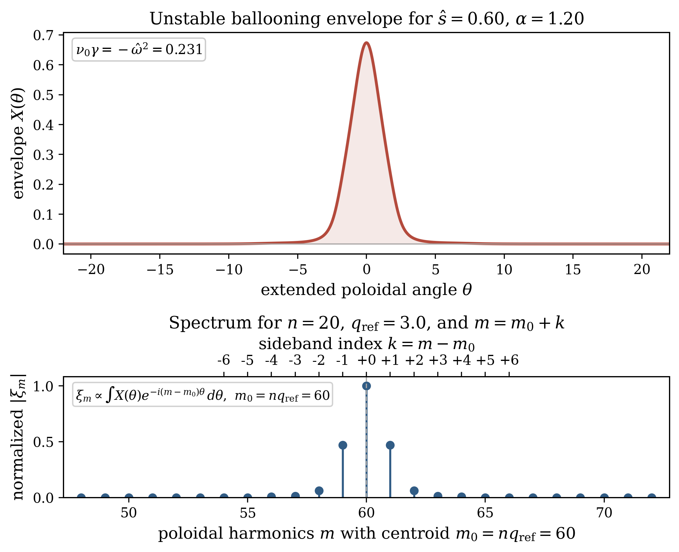
Choice of \(n\) and interpretation of the \(m\) spectrum
The field-line envelope \(X(\theta )\) is the high-\(n\) ballooning object. It does not represent one isolated Fourier harmonic;
instead it reconstructs a packet of poloidal sidebands with \(m\simeq nq\). For illustration we choose a large but finite
toroidal mode number \(n=20\) and a reference safety factor \(q_{\rm ref}=3.0\) on the chosen reference surface, so the packet
is centered on \[ m_0 \approx n q_{\rm ref} = 20\times 3.0 \approx 60. \] Writing \[ m = m_0 + k, \] the ballooning transform implies that the sideband amplitudes are
obtained from the Fourier content of the envelope through \[ \xi _m \propto \int _{-\infty }^{\infty } X(\theta )e^{-ik\theta }\,d\theta , \qquad k = m-m_0. \] The envelope therefore brackets a
narrow packet of neighboring \(m\) values around the centroid \(m_0\), rather than selecting one isolated \((m,n)\)
harmonic.
Representative unstable example
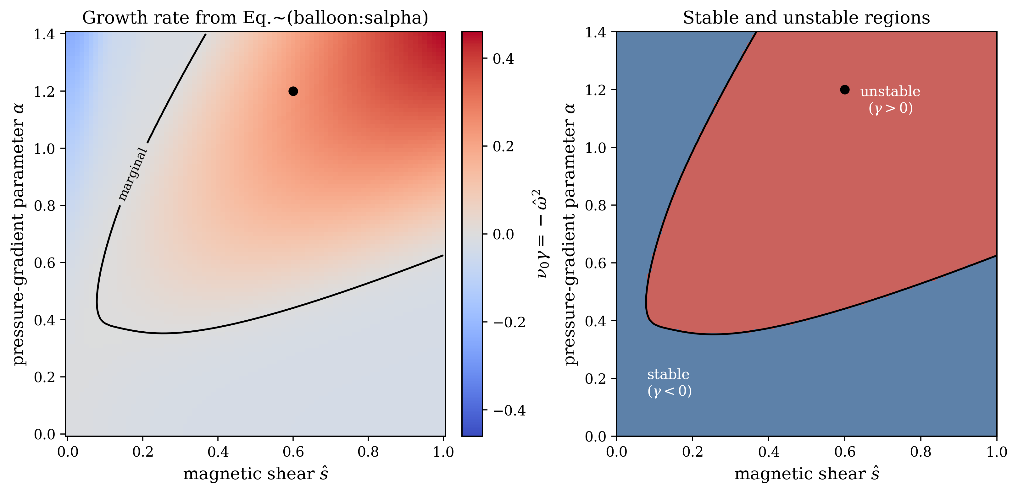
For the example shown in Fig. 26.1 we use \(\hat s=0.60\) and \(\alpha =1.20\), which gives \[ \nu _0\gamma = -\hat \omega ^2 \approx 0.231. \] This point lies inside the unstable region of
the \(\hat s\)–\(\alpha \) diagram and produces a strongly localized outboard ballooning envelope.
The general growth-rate map and the stable/unstable partition obtained from the same numerical
eigensolver are shown in Fig. 26.2.
Reading the equation term by term
Equation (26.86) looks complicated at first glance, but its logic is simple.
If \(\alpha =0\), there is no pressure-gradient drive and the equation contains only stabilizing pieces. If \(\hat s\) is increased at
fixed pressure gradient, the factor \(1+\Lambda ^2\) grows more rapidly away from the outboard side, so the mode pays a
stronger shear-generated bending penalty. And because the coefficient multiplying \(X\) changes sign around
the torus, the mode finds it energetically favorable to concentrate where the curvature is bad and to avoid
where it is good.
That is the entire subject in one sentence: ballooning is toroidal buoyancy localized by shear and opposed by
line bending.
A local expansion near the outboard side
Near \(\theta =0\) one has
\[\cos \theta \simeq 1-\frac {\theta ^2}{2}, \qquad \Lambda \simeq \hat s\,\theta .\]
Then the reduced equation behaves like a one-dimensional bound-state problem: the curvature term makes
a potential well centered at the outboard side, while magnetic shear makes the well narrower by increasing
the stiffness away from \(\theta =0\). This is a crude analogy, but it is a very good one. The ballooning eigenfunction is
a bound state created by toroidal buoyancy.
Rayleigh quotient and the sign of the mode
Multiplying (26.86) by \(X\) and integrating by parts gives
\[\delta W[X] = \hat \omega ^2\mathcal N[X]. \tag{26.88}\]
Since \(\mathcal N[X]>0\), instability is equivalent to \[\delta W[X]<0 \qquad \Longleftrightarrow \qquad \hat \omega ^2<0.\]
In the drag formulation (26.68), the same condition is \(\gamma >0\), because Eq. (26.81) gives \(\nu _0\gamma =-\hat \omega ^2\). So the wave problem,
the energy principle, and the Ham sliding-tube linearization are not three different stories. They are the
same story written in three different languages.
27.6 What ballooning adds beyond interchange
Mercier, Suydam, and the high-\(n\) limit
There is a useful hierarchy here. Suydam and Mercier ask whether an equilibrium is locally vulnerable to
interchange-like distortions once shear and compressibility are taken into account. Ballooning theory then
asks a sharper question: if the plasma is allowed to choose where along a toroidal field line it will
bulge, what is the most dangerous localization it can find? In that sense ballooning theory is
not a separate instability from interchange. It is the high-\(n\), toroidally localized refinement of
interchange.
This is why the connection to buoyancy is so important. If one forgets the buoyancy picture, the \(\hat s\)–\(\alpha \)
equation can look like a mysterious toroidal differential equation. If one remembers it, the meaning of the
equation is immediate: it is the optimal competition between bad-curvature buoyancy and line-bending
stabilization on a sheared field.
First and second stability
One of the classic lessons of ballooning theory is that increasing pressure gradient does not produce a
single monotone stability boundary. For some combinations of shaping and shear, a tokamak can pass
through a first unstable ballooning region and then re-enter a second stable region at higher pressure
Strauss et al. (1980); Freidberg (1982). The reason is now easy to state in words: toroidal buoyancy is
trying to drive the mode, but the same toroidal geometry also changes the way the mode bends the field.
So the equilibrium can become unstable and then stable again as the geometry of the best localized
eigenfunction changes.
The flux-tube viewpoint
The later nonlinear flux-tube picture is worth mentioning even in a linear lecture. Instead of treating
ballooning as an abstract eigenfunction problem, one imagines a narrow tube sliding on a Clebsch surface,
feeling a generalized Archimedes force of the type in (26.14), while field-line bending and shear constrain
the trajectory. The linear ballooning equation is then the small-amplitude limit of a much richer nonlinear
problem. The eigenfunction is not just a mathematical object. It is the infinitesimal version of a real
erupting flux tube.
Takeaways
-
1.
- Ballooning is the toroidal descendant of buoyancy and interchange, not a wholly
new kind of drive.
-
2.
- A thin displaced flux tube feels a generalized Archimedes force \(F_n\simeq 2A\kappa _n(p_{\rm in}-p_0)\), which becomes
destabilizing on the outboard side because \(\dd {p_0}{r}<0\) and \(\kappa _n>0\) there.
-
3.
- The local force balance \(\omega ^2=v_A^2k_{\parallel }^2 + 2\kappa _n\rho ^{-1}\dd {p_0}{r}\) is the toroidal analog of the Brunt–Väisälä oscillator.
-
4.
- Magnetic shear makes \(k_x\simeq k_y\hat s\theta \), so a mode cannot remain cheap everywhere along a field
line. It localizes where the buoyancy drive is strongest.
-
5.
- The \(\hat s\)–\(\alpha \) equation is simply the reduced Euler–Lagrange equation of that
one-dimensional variational problem.
-
6.
- The Cowley–Ham sliding-tube equation promotes the linear displacement to a
finite field-line shape \(r(\theta ,r_0,t)\), while preserving the same geometric factor \(1+(\alpha \sin \theta -\hat s\theta )^2\) that measures
shear-amplified line bending.
Bibliography
Harold P. Furth, John Killeen, and Marshall N. Rosenbluth. Finite-resistivity instabilities of a sheet pinch. Physics of Fluids, 6(4):459–484, 1963. doi:10.1063/1.1706761.
Bruno Coppi, John M. Greene, and John L. Johnson. Resistive instabilities in a diffuse linear pinch. Nuclear Fusion, 6(2):101–117, 1966. doi:10.1088/0029-5515/6/2/003.
P. H. Rutherford. Nonlinear growth of the tearing mode. Physics of Fluids, 16(11):1903–1908, 1973.
B. B. Kadomtsev. Disruptive instability in tokamaks. Soviet Journal of Plasma Physics, 1:389–391, 1975. English translation of Fizika Plazmy 1, 710 (1975).
C. C. Hegna. The physics of neoclassical magnetohydrodynamic tearing modes. Physics of Plasmas, 5(5):1767–1774, 1998. doi:10.1063/1.872846.
R. J. La Haye. Neoclassical tearing modes and their control. Physics of Plasmas, 13(5):055501, 2006. doi:10.1063/1.2180747.
R. J. La Haye, R. Fitzpatrick, T. C. Hender, A. W. Morris, J. T. Scoville, and T. N. Todd. Critical error fields for locked mode instability in tokamaks. Physics of Fluids B: Plasma Physics, 4(7):2098–2103, 1992. doi:10.1063/1.860017.
C. C. Hegna and J. D. Callen. On the stabilization of neoclassical magnetohydrodynamic tearing modes using localized current drive or heating. Physics of Plasmas, 4(8):2940–2946, 1997. doi:10.1063/1.872426.
E. Lazzaro, R. J. Buttery, T. C. Hender, P. Zanca, R. Fitzpatrick, M. Bigi, T. Bolzonella, R. Coelho, M. DeBenedetti, S. Nowak, O. Sauter, and M. Stamp. Error field locked modes thresholds in rotating plasmas, anomalous braking and spin-up. Physics of Plasmas, 9(9):3906–3918, 2002. doi:10.1063/1.1499495.
R. Fitzpatrick. Interaction of tearing modes with external structures in cylindrical geometry. Nuclear Fusion, 33(7):1049–1084, 1993. doi:10.1088/0029-5515/33/7/I08.
Alexander B. Rechester and Thomas H. Stix. Magnetic braiding due to weak asymmetry. Physical Review Letters, 36(11):587–591, 1976. doi:10.1103/PhysRevLett.36.587.
Alexander B. Rechester and Marshall N. Rosenbluth. Electron heat transport in a tokamak with destroyed magnetic surfaces. Physical Review Letters, 40(1):38–41, 1978. doi:10.1103/PhysRevLett.40.38.
T. M. Biewer, C. B. Forest, J. K. Anderson, G. Fiksel, B. Hudson, S. C. Prager, J. S. Sarff, J. C. Wright, D. L. Brower, W. X. Ding, and S. D. Terry. Electron heat transport measured in a stochastic magnetic field. Physical Review Letters, 91(4):045004, 2003. doi:10.1103/PhysRevLett.91.045004.
R Oâ O'Connell, D J Den Hartog, C B Forest, J K Anderson, T M Biewer, B E Chapman, D Craig, G Fiksel, S C Prager, J S Sarff, S D Terry, and R W Harvey. Observation of velocity-independent electron transport in the reversed field pinch. Physical Review Letters, 91(4):045002, 2003. ISSN 0031-9007. doi:10.1103/physrevlett.91.045002.
J. A. Reusch, J. K. Anderson, D. J. Den Hartog, F. Ebrahimi, D. D. Schnack, H. D. Stephens, and C. B. Forest. Experimental evidence for a reduction in electron thermal diffusion due to trapped particles. Physical Review Letters, 107(15):155002, 2011. doi:10.1103/PhysRevLett.107.155002.
Benjamin D. G. Chandran and Steven C. Cowley. Thermal conduction in a tangled magnetic field. Physical Review Letters, 80(14):3077–3080, 1998. doi:10.1103/PhysRevLett.80.3077.
Benjamin D. G. Chandran, Steven C. Cowley, Mariya Ivanushkina, and Richard Sydora. Heat transport along an inhomogeneous magnetic field. I. periodic magnetic mirrors. The Astrophysical Journal, 525(2):638–650, 1999. doi:10.1086/307915.
B. Coppi, R. Galv ao, R. Pellat, M. N. Rosenbluth, and P. H. Rutherford. Resistive internal kink modes. Soviet Journal of Plasma Physics, 2:533–535, 1976. Translated from Fizika Plazmy 2, 961–966 (1976).
G. Ara, B. Basu, B. Coppi, G. Laval, M. N. Rosenbluth, and B. V. Waddell. Magnetic reconnection and $m=1$ oscillations in current carrying plasmas. Annals of Physics, 112(2):443–476, 1978. doi:10.1016/S0003-4916(78)80007-4.
S. Migliuolo. Theory of ideal and resistive $m=1$ modes in tokamaks. Nuclear Fusion, 33(11):1721–1754, 1993. doi:10.1088/0029-5515/33/11/I13.
N. F. Loureiro, A. A. Schekochihin, and S. C. Cowley. Instability of current sheets and formation of plasmoid chains. Physics of Plasmas, 14(10):100703, 2007. doi:10.1063/1.2783986.
Claude Mercier. A necessary condition for hydromagnetic stability of plasma with axial symmetry. Nuclear Fusion, 1(1):47–53, 1960. doi:10.1088/0029-5515/1/1/004.
J. W. Connor, R. J. Hastie, and J. B. Taylor. Shear, periodicity, and plasma ballooning modes. Physical Review Letters, 40(6):396–399, 1978. doi:10.1103/PhysRevLett.40.396.
H. R. Strauss, W. Park, D. A. Monticello, R. B. White, S. C. Jardin, M. S. Chance, A. M. M. Todd, and A. H. Glasser. Stability of high-beta tokamaks to ballooning modes. Nuclear Fusion, 20(5):638–642, 1980. doi:10.1088/0029-5515/20/5/014.
C. J. Ham, S. C. Cowley, G. Brochard, and H. R. Wilson. Nonlinear stability and saturation of ballooning modes in tokamaks*. Physical Review Letters, 116(23):235001, 2016. ISSN 0031-9007. doi:10.1103/physrevlett.116.235001.
A. M. M. Todd, M. S. Chance, J. M. Greene, R. C. Grimm, J. L. Johnson, and J. Manickam. Stability limitations on high-beta tokamaks. Physical Review Letters, 38(15):826–829, 1977. doi:10.1103/PhysRevLett.38.826.
D. Dobrott, D. B. Nelson, J. M. Greene, A. H. Glasser, M. S. Chance, and E. A. Frieman. Theory of ballooning modes in tokamaks with finite shear. Physical Review Letters, 39(15):943–946, 1977. doi:10.1103/PhysRevLett.39.943.
J. W. Connor, R. J. Hastie, and J. B. Taylor. High mode number stability of an axisymmetric toroidal plasma. Proceedings of the Royal Society of London. Series A. Mathematical and Physical Sciences, 365(1720):1–17, 1979. doi:10.1098/rspa.1979.0001.
B. Coppi. Topology of ballooning modes. Physical Review Letters, 39(15):939–942, 1977. doi:10.1103/PhysRevLett.39.939.
J. P. Freidberg. Ideal magnetohydrodynamic theory of magnetic fusion systems. Reviews of Modern Physics, 54(3):801–902, 1982. doi:10.1103/RevModPhys.54.801.
Problems
-
Problem 27.1.
- Starting from the force balance (26.19), show directly that for a large-aspect-ratio
tokamak the curvature term can be written in the form \(\rho N_{\rm tor}^2(\theta )\xi _n\) with (26.27). Identify
explicitly the regions of good and bad curvature.
-
Problem 27.2.
- Derive (26.14) from the pressure-balance condition (26.12). Then linearize to
obtain (26.16). Explain in words why the sign changes between the outboard and
inboard sides of the torus.
-
Problem 27.3.
- Starting from \(\chi =\zeta -q(r)\theta \), derive (26.33). Then estimate how the bending energy in (26.36)
changes with increasing \(|\theta |\) and explain why a mode centered at the outboard
midplane becomes localized.
-
Problem 27.4.
- Take the reduced functional (26.70) together with the norm (26.72) and rederive
the ballooning equation (26.86) by varying \(\delta W[X]-\hat \omega ^2\mathcal N[X]\). Be careful with the boundary term
at \(|\theta |\rightarrow \infty \).
-
Problem 27.5.
- Using the physical interpretation of the coefficients in (26.86), explain qualitatively
how a tokamak can pass from stability to instability and then back to stability
as \(\alpha \) is increased at fixed shear. What ingredients of toroidal geometry make such
behavior possible?
-
Problem 27.6.
- Starting from (26.65), set \(r(\theta ,r_0,t)=r_0+\xi (\theta ,t)\) and keep only terms linear in \(\xi \). Show that the nonlinear
buoyancy term gives \(\alpha (r_0)[\cos \theta +\sin \theta (s_0\theta -\alpha (r_0)\sin \theta )]\xi \) and that the last term in (26.65) is quadratic. Recover
(26.68).