Lecture 29
Coppi, Greene, and Johnson: Resistive Interchange
Overview
Resistive interchange is the natural bridge between the local buoyancy arguments of
Suydam and the reconnection physics of the tearing lecture. The regime we want to
isolate is deliberately subtle: the plasma is tearing stable in the outer-region sense, so
that the classical magnetic matching parameter satisfies \(\Delta '<0\), and it is also Suydam stable,
so that the local ideal singularity is below threshold. Thus neither ordinary FKR tearing
nor ideal interchange is allowed to explain the mode.
That is exactly why the Coppi–Greene–Johnson problem is so useful. Once the ideal
Suydam problem is stable, the outer-region radial displacement near the resonant surface
is already known as a Frobenius solution. The job of the resistive layer is not to invent
a new outer solution; it is to produce an inner solution for \(\xi _r\) that can be matched to that
Suydam form. The surprising result is that a pressure-gradient drive inside the layer can
still produce a growing, island-forming branch even when \(\Delta '\) is unfavorable.
The key lesson is that two parity classes are present. One is interchange-like, with a
finite radial displacement at the resonant surface but vanishing helical flux there. The
other is tearing-like, with finite helical flux at the surface and therefore genuine island
formation. In the second case a plasma can be stable according to the classical outer
tearing index \(\Delta '\) and yet still develop islands because pressure gradients in a low-shear
layer do part of the destabilizing work.
Historical Perspective
The sheet-pinch paper of Furth, Killeen, and Rosenbluth made the matched-asymptotic
idea famous: ideal MHD outside, a narrow resistive layer inside Furth et al. (1963).
Coppi, Greene, and Johnson then carried that logic into the diffuse linear pinch, where
the equilibrium curvature is cylindrical rather than gravitational and finite pressure
can no longer be ignored Coppi et al. (1966). Their paper is still remarkable for how
explicitly it refuses to draw hard category lines: “interchange,” “kink,” and “tearing” are
shown to be closely related limits of the same resistive-layer problem.
That old lesson has aged very well. In modern tokamak language, the low-shear
pressure-driven \((m,n)=(1,1)\) structures discussed in hybrid and sawtooth-free plasmas Stober
et al. (2007) are best thought of as descendants of this same resistive-interchange /
quasi-interchange family. The geometry is now toroidal and the nonlinear saturation is
far richer, but the analytic seed is already present in the cylindrical problem Jardin
et al. (2015); Krebs et al. (2017).
Caution
Three distinctions are easy to blur.
First, \(\Delta '\) is an outer matching index. It measures how the ideal solution leans into an inner
layer, just as in the tearing lecture, Eq. (27.2). It does not by itself know about local
pressure-gradient drive.
Second, Suydam’s criterion, Eq. (23.17), is an ideal local criterion. Passing it only says
that the ideal singularity is mild enough to be regularized without an immediate ideal
interchange catastrophe. It does not say that the resistive problem is stable.
Third, Coppi’s “even” and “odd” labels refer to the parity of the radial displacement \(\bar {\xi }_r\),
not the parity of the perturbed flux \(\psi \). Since the two have opposite parity in the layer
equations, this matters.
29.1 The resistive window left open by Suydam
The outer ideal problem is still the Newcomb problem developed in the diffuse-pinch lecture, with local
resonant surface defined by
\[F(r) \equiv \frac {mB_\theta (r)}{r} + k B_z(r)=0, \qquad k=-\frac {n}{R_0}. \tag{28.1}\]
At such a surface, the local ideal energy functional reduced in Eq. (23.8) gives the dimensionless
pressure-drive parameter \[D_s \equiv -\frac {2\muo k^2}{r_s[F'(r_s)]^2}\,p'(r_s) = -\frac {2\muo q_s^2}{r_s B_z^2(r_s)\,[q_s'(r_s)]^2}\,p'(r_s), \tag{28.2}\]
which was already used to write Suydam’s criterion in the form \[D_s \le \frac 14. \tag{28.3}\]
The physically interesting regime for this lecture is not the ideal-interchange regime \(D_s>1/4\), and it is not the
classical tearing regime \(\Delta '>0\). We will instead keep the two stability assumptions \[\Delta '<0, \qquad 0<D_s<\frac 14 . \tag{28.4}\]
The pressure decreases outward, so the curvature/pressure combination is destabilizing, but magnetic
shear is still strong enough that ideal MHD remains locally regular. The current profile is also chosen so
that the ordinary outer tearing mode is stable.
Why flat shear matters.
Equation (28.2) says it plainly:
\[D_s \propto \frac {|p'(r_s)|}{[q_s'(r_s)]^2}. \tag{28.5}\]
Thus a mild pressure gradient can become important if the magnetic shear is sufficiently small. That is the
first conceptual connection to the gravitational-interchange lecture. In both cases there is a buoyancy-like
drive; in the cylindrical plasma it is magnetic curvature rather than true gravity, and the quantity that
opposes it is not just field strength but field-line shear.
The outer solution is already fixed.
Near the resonant surface write
\[x \equiv r-r_s.\]
The local ideal equation then reduces to the Suydam form \[\dd {}{x}\left (x^2\dd {\xi _r}{x}\right )+D_s\,\xi _r=0. \tag{28.7}\]
Let \[h\equiv \frac 12\left [\sqrt {1-4D_s}-1\right ], \qquad -\frac 12<h<0 \qquad (0<D_s<1/4). \tag{28.8}\]
Then, on either side of the layer, the ideal outer displacement has the Coppi–Greene–Johnson form
\[\xi _{r,\rm out}^{\pm }(x) = c_1^{\pm }\left |\frac {x}{r_s}\right |^{h} + c_2^{\pm }\left |\frac {x}{r_s}\right |^{-1-h}, \qquad \pm x>0. \tag{28.9}\]
Equivalently, \[\xi _r \sim |x|^{p_\pm }, \qquad p_\pm =\frac {-1\pm \sqrt {1-4D_s}}{2}, \tag{28.10}\]
with \(p_+=h\) and \(p_-=-1-h\). This is the main point to keep in view: because the plasma is Suydam stable, the outer
problem does not blow up into an ideal interchange catastrophe. We can therefore write the outer solution
immediately. The inner resistive-layer solution for \(\Xi (X)\), derived below, must later be matched to the two
coefficients \(c_1^\pm \) and \(c_2^\pm \).
This is also where \(\Delta '\) and Suydam stability separate cleanly. The \(\Delta '\)-stable condition controls the outer
helical-flux matching used in the tearing lecture. Equation (28.9) controls the outer displacement matching
used by the pressure-driven layer. Resistive interchange becomes possible because those are different pieces
of the same global eigenfunction.
29.2 Reduced layer equations
The layer calculation uses the same resonant geometry as tearing, but it cannot be closed with the
induction equation and perpendicular vorticity equation alone. In finite-pressure cylindrical geometry the
magnetic perturbation parallel to the equilibrium field is a dynamical part of the layer. This is the point
that is easy to hide if one jumps too quickly to a two-field model.
Layer scales.
Near the rational surface,
\[F(r) \simeq F_s' x, \qquad x\equiv r-r_s, \qquad k_\parallel (x)\simeq \frac {F_s'}{B_s}x. \tag{28.11}\]
Write \[\eta _m\equiv \frac {\eta }{\muo }, \qquad k_\perp \equiv \frac {m}{r_s}, \qquad L_s\equiv \left |\frac {q_s}{q_s'}\right |.\]
Equivalently, \(k_\parallel \simeq k_\perp \mathcal {F}_s' x\), with \(\mathcal {F}_s'\equiv (q'/q)_s\) as a signed shear. The inner induction balance is the same resistive skin-depth
balance used in tearing, \[d_R^2\sim \frac {\eta _m}{\gamma _R}. \tag{28.13}\]
The difference is in the force balance. In the interchange ordering, inertia balances the field-line-bending
force \(\rho \gamma ^2 \xi \sim k_\parallel ^2 B^2 \xi \)
evaluated inside the layer: \[\gamma _R^2 \sim V_A^2 k_\parallel ^2(d_R) \sim V_A^2 k_\perp ^2\frac {d_R^2}{L_s^2}, \qquad V_A\equiv \frac {B_s}{\sqrt {\muo \rho _s}} . \tag{28.14}\]
Combining Eqs. (28.13) and (28.14) gives the natural resistive-interchange scales \[\gamma _R \equiv \left (\eta _m\frac {k_\perp ^2V_A^2}{L_s^2}\right )^{1/3}\sim \frac {1}{\tau _R^{1/3}\tau _A^{2/3}}, \qquad d_R \equiv \left (\frac {\eta _m}{\gamma _R}\right )^{1/2} = \left (\frac {\eta _m L_s}{k_\perp V_A}\right )^{1/3} \left (\frac {a}{L_s}\right )^{1/3}. \tag{28.15}\]
These are the scales behind the familiar \(\eta ^{1/3}\) resistive-interchange growth law. The dimensionless eigenvalue is
not determined by this scaling argument; it comes from solving and matching the layer equations
below.
Use physical parallel variables.
Coppi, Greene, and Johnson decompose vectors using the non-unit basis vector \(\B _0\). That is compact, but it
hides the units: their coefficient multiplying \(\B _0\) is not itself a physical displacement or a physical magnetic
perturbation. We will make the parallel pieces explicit by writing
\[\boldsymbol {\xi } = \xi \,\hat {\mathbf r} +\xi _\parallel \,\hat {\mathbf b} +\xi _\perp \,(\hat {\mathbf r}\times \hat {\mathbf b}), \qquad \B _1 = b_r\,\hat {\mathbf r} +b_\parallel \,\hat {\mathbf b} +b_\perp \,(\hat {\mathbf r}\times \hat {\mathbf b}), \tag{28.16}\]
where \(\hat {\mathbf b}=\B _0/B_s\). The ambiguous \(b_b\) subscript in the printed version of their Eq. (49) should be read as the
same parallel magnetic perturbation. The one-time translation from the original notation is
\[\xi _\parallel = B_s\,\xi _B, \qquad b_\parallel = B_s\,b_B. \tag{28.17}\]
After Eq. (28.17), the layer algebra below uses only \(\xi _\parallel \) and \(b_\parallel \). We also drop CGJ’s order labels \((0)\), \((1)\), and \((2)\).
All quantities in Eqs. (48)–(52) below are the leading nonzero pieces in the slow-interchange
ordering.
Total-pressure balance and the new parallel equation.
We now write the local layer equations directly in SI units. The linearized momentum equation is
\[\rho \gamma ^2\boldsymbol {\xi } = -\nabla p_1 + \frac {1}{\muo }\left [(\nabla \times \B _1)\times \B _0+(\nabla \times \B _0)\times \B _1\right ], \tag{28.18}\]
and the induction equation is \[\B _1-\frac {\eta _m}{\gamma }\nabla ^2\B _1 = \nabla \times (\boldsymbol {\xi }\times \B _0), \qquad \eta _m\equiv \frac {\eta }{\muo }. \tag{28.19}\]
Here \(\eta \) is the electrical resistivity and \(\eta _m\) is the magnetic diffusivity. The symbol \(\gamma \) is the growth rate; the safety
factor remains \(q(r)\).
The fast magnetosonic response across the layer enforces near constancy of total pressure,
\[p_1+\frac {B_s b_\parallel }{\muo }\simeq 0 . \tag{28.20}\]
The adiabatic pressure equation gives \[p_1=-p'\xi -\Gamma p\,\nabla \cdot \boldsymbol {\xi }, \tag{28.21}\]
where \(\Gamma \) is the ratio of specific heats and all equilibrium quantities are evaluated at \(r=r_s\). Combining
Eqs. (28.20) and (28.21) gives the SI version of the CGJ total-pressure relation, \[\frac {B_s b_\parallel }{\muo } = p'\xi +\Gamma p\,\nabla \cdot \boldsymbol {\xi }. \tag{48}\]
This relation is not optional: without Eq. (48), one cannot eliminate the compressive part of the motion
and one does not obtain the correct third layer equation.
Deriving the parallel-displacement equation.
The parallel displacement enters because finite pressure permits a slow, sound-like adjustment along the
resonant field line. Project Eq. (28.18) along \(\hat {\mathbf b}\). The term \((\nabla \times \B _1)\times \B _0\) is perpendicular to \(\B _0\), so it drops out of this
projection. The remaining equilibrium-current term may be written using force balance. Since
\[\frac {1}{\muo }(\nabla \times \B _0)\times \B _0=\nabla p,\]
the perpendicular part of the equilibrium current satisfies \[\hat {\mathbf b}\times \mathbf {J}_0=-\frac {\nabla p}{B_s}, \qquad \mathbf {J}_0\equiv \frac {\nabla \times \B _0}{\muo }. \tag{28.23}\]
Therefore \[\hat {\mathbf b}\cdot (\mathbf {J}_0\times \B _1) = \B _1\cdot (\hat {\mathbf b}\times \mathbf {J}_0) = -\frac {p'}{B_s}\,b_r . \tag{28.24}\]
The pressure-gradient term along the field is handled with total-pressure balance: \[-\nabla _\parallel p_1 \simeq \frac {B_s}{\muo }\nabla _\parallel b_\parallel . \tag{28.25}\]
Near the rational surface, \[k_\parallel (x)\simeq k_\perp \mathcal {F}_s' x, \qquad k_\perp \equiv \frac {m}{r_s}, \qquad \mathcal {F}_s'\equiv \left (\frac {q'}{q}\right )_s, \tag{28.26}\]
up to the sign convention used for the helicity. Equivalently, in the rotational-transform notation used by
CGJ, \[\frac {mB_s\mathcal {F}_s'}{r_s}x = \frac {m k B_z\iota _s'}{2\pi }x . \tag{28.27}\]
Thus \(\nabla _\parallel b_\parallel \simeq \mathrm {i}k_\parallel b_\parallel \), and the parallel component of the equation of motion becomes \[\rho \gamma ^2\xi _\parallel = -\frac {p'}{B_s}\,b_r + \frac {\mathrm {i}B_s}{\muo }k_\parallel (x)b_\parallel = -\frac {p'}{B_s}\,b_r + \frac {\mathrm {i}mB_s\mathcal {F}_s'}{\muo r_s}\,x b_\parallel . \tag{49}\]
This is the cleaned-up SI form of CGJ Eq. (49). It says that \(\xi _\parallel \) is not an extra closure assumption; it is
determined by the parallel force balance between the pressure-gradient force associated with \(b_r\) and the
resonant-field-line force associated with \(b_\parallel \).
Where CGJ Eq. (52) comes from.
Take the component of Eq. (28.19) parallel to \(\B _0\). Using
\[\nabla \times (\boldsymbol {\xi }\times \B _0) = (\B _0\cdot \nabla )\boldsymbol {\xi } - (\boldsymbol {\xi }\cdot \nabla )\B _0 - \B _0\nabla \cdot \boldsymbol {\xi }, \tag{28.28}\]
and keeping the leading layer derivatives gives \[b_\parallel -\frac {\eta _m}{\gamma }\,b_\parallel '' = \mathrm {i}B_s k_\parallel (x)\xi _\parallel - B_s\nabla \cdot \boldsymbol {\xi } - \frac {(\muo p+B^2)'}{B_s}\,\xi . \tag{52}\]
The three terms on the right have distinct origins. The first is parallel stretching of the magnetic field by \(\xi _\parallel \).
The second is compression. The third is the convective change of the equilibrium total-pressure constraint;
in SI the combination that has the units of magnetic pressure is \(\muo p+B^2\). This is the equation that is absent from a
two-field tearing derivation.
Now use Eq. (48) to eliminate the divergence,
\[\nabla \cdot \boldsymbol {\xi } = \frac {1}{\Gamma p}\left (\frac {B_s b_\parallel }{\muo }-p'\xi \right ) = \frac {2}{\Gamma \beta }\frac {b_\parallel }{B_s} - \frac {2\muo p'}{\Gamma \beta B_s^2}\xi , \qquad \beta \equiv \frac {2\muo p}{B_s^2}. \tag{28.29}\]
Then use Eq. (49) to eliminate \(\xi _\parallel \). This is the direct route from CGJ Eq. (52) to their normalized Eq. (62),
but now every variable has ordinary SI units.
Normalized CGJ variables.
The CGJ scale length and frequency are just the resistive-interchange layer width and rate. We therefore
write them as \(d_R\) and \(\gamma _R\),
\[\gamma _R \equiv \left (\eta _m\frac {m^2(\mathcal {F}_s')^2V_A^2}{r_s^2}\right )^{1/3}, \qquad d_R \equiv \left (\frac {\eta _m}{\gamma _R}\right )^{1/2} = \left (\frac {\eta _m^2 r_s^2}{m^2(\mathcal {F}_s')^2V_A^2}\right )^{1/6}, \qquad V_A\equiv \frac {B_s}{\sqrt {\muo \rho }} . \tag{28.30}\]
These are the SI versions of the scale length and scale frequency used by CGJ. Define \[X\equiv \frac {x}{d_R}, \qquad Q\equiv \frac {\gamma }{\gamma _R}, \qquad \Xi \equiv \xi , \tag{28.31}\]
and \[\Psi \equiv \frac {\mathrm {i} r_s}{d_R m\mathcal {F}_s' B_s}\,b_r, \qquad \Upsilon \equiv \frac {D B_s}{\muo p'}\,b_\parallel . \tag{28.32}\]
Here \(D\) is the same Suydam drive parameter as \(D_s\), evaluated at the resonant surface, and \(\Upsilon \) is proportional to
the parallel magnetic-field perturbation. It is not an independent pressure variable. Finally,
\[\mathcal {S}\equiv -\frac {2B_\theta ^2D}{\muo r_s p'} \tag{28.33}\]
is a stabilizing geometric term. Primes on \(\Psi \), \(\Xi \), and \(\Upsilon \) below denote \(d/dX\).
This coefficient deserves a little motivation because it is easy to treat it as a formal symbol. Using
Eq. (28.2) together with the cylindrical relation
\[q_s=\frac {r_s B_z(r_s)}{R_0 B_\theta (r_s)},\]
one may rewrite Eq. (28.33) as \[\mathcal {S} = \frac {4}{R_0^2[q_s'(r_s)]^2}. \tag{28.35}\]
Thus \(\mathcal S\) is controlled by the same low-shear geometry that makes \(D_s\) important in the first place. If \(q_s\sim O(1)\) and the
shear length \(L_s=q_s/q_s'\) is a substantial fraction of the major radius, then \(\mathcal S\sim O(1)\). That is why finite-\(\beta \) comparisons with \(\mathcal S=0\) and
\(\mathcal S\sim 1\) are both worth examining: the former isolates the compressibility effect, while the latter is closer to the
natural cylindrical estimate.
The three equations to solve.
The radial induction equation gives
\[\Psi ''=Q(\Psi +X\Xi ). \tag{60}\]
The annihilated perpendicular equation of motion gives \[\Xi '' = \frac {X^2}{Q}\,\Xi + \frac {X}{Q}\,\Psi - \frac {1}{Q^2}\,\Upsilon . \tag{61}\]
The parallel induction equation, Eq. (52), after using Eqs. (28.29) and (49), gives \[\Upsilon '' = Q\left (1+\frac {X^2}{Q^2}+\frac {2}{\Gamma \beta }\right )\Upsilon + Q\left (\mathcal {S}-D-\frac {2D}{\Gamma \beta }\right )\Xi + \frac {D}{Q}\,X\Psi . \tag{62}\]
These are the central equations of the lecture. Equation (60) is the same resistive induction balance that
appears in tearing, Eq. (61) is the radial equation of motion, and Eq. (62) is the new finite-pressure
equation for the parallel magnetic perturbation \(b_\parallel \). The pressure drive is distributed through \(\Upsilon \), \(D\), and \(\mathcal S\); it is
not a simple additive correction to \(\Delta '\).
Caution
The signs of the \(X\Xi \) and \(X\Psi \) terms depend on the sign convention used for \(\Psi \) and for the
signed shear \(\mathcal {F}_s'\). The convention above follows Coppi, Greene, and Johnson. Reversing the
definition of \(\Psi \) flips those two signs but leaves the eigenvalue problem unchanged.
Low-\(\beta \) reduction.
When \(\beta \ll 1\), Eq. (62) forces the leading balance
\[\Upsilon \simeq D\Xi . \tag{28.36}\]
Substituting this into Eq. (61) leaves the familiar two-field low-\(\beta \) resistive-interchange model,
\[\Psi ''=Q(\Psi +X\Xi ), \tag{28.37}\]
\[\Xi '' = \frac {X^2}{Q}\,\Xi + \frac {X}{Q}\,\Psi - \frac {D}{Q^2}\,\Xi . \tag{28.38}\]
This reduced system is useful for intuition, but the three-field system (60)–(62) is the one we should regard
as the complete finite-pressure layer problem.
A useful way to think about this reduction is as a formal organizing limit. If \(\beta \ll 1\) and one begins from the
singular small-\(Q\) limit, then Eq. (62) collapses to \(\Upsilon \simeq D\Xi \) and the two parity classes are nearly degenerate. But \(Q=0\) is
not the physical eigenvalue. The actual matched low-\(\beta \) problem still selects a finite \(Q\), and for the standard
Coppi benchmark at \(D_s=3/16\) that value is
\[Q \simeq 0.39685. \tag{28.39}\]
So the small-\(\beta \), small-\(Q\) limit is best viewed as the point from which the parity pair is organized, not as the
final growth rate.
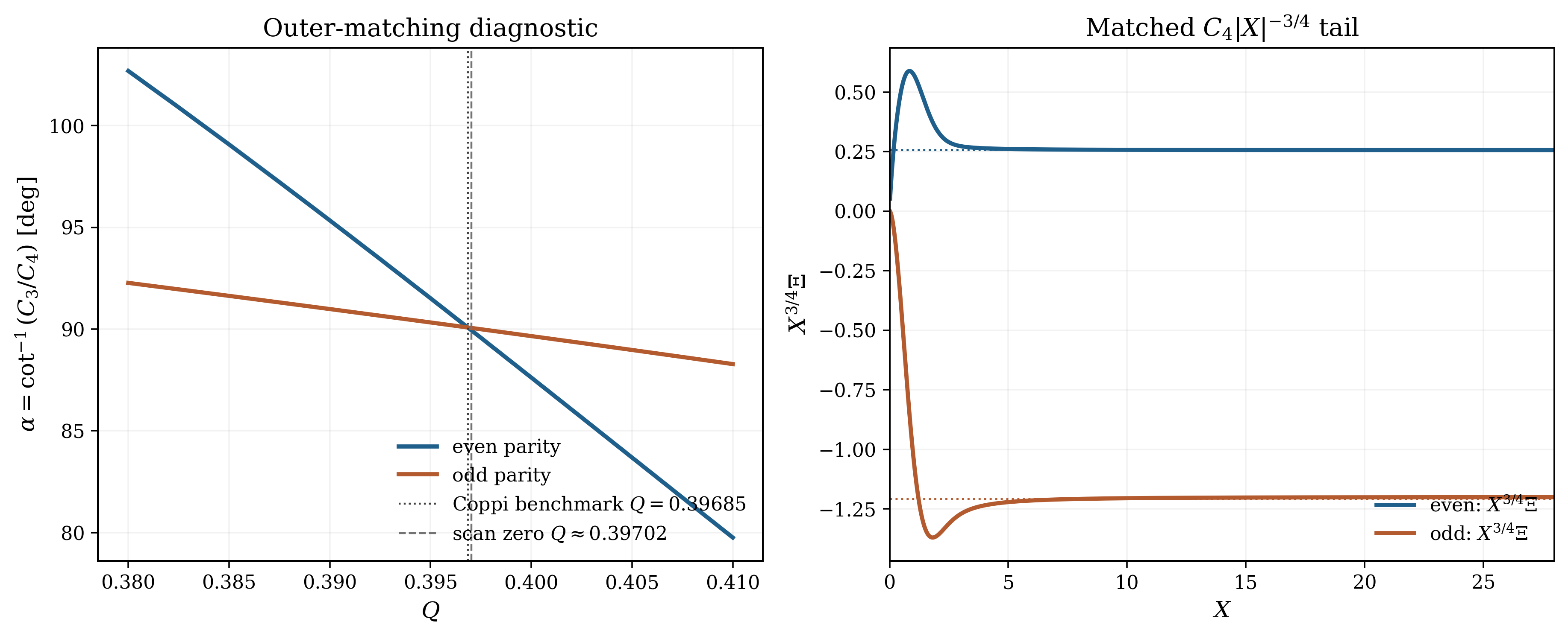
Matching to the Suydam outer solution.
For \(|X|\gg 1\), the non-exponentially-growing part of the inner solution for \(\Xi \) has the same two Suydam powers as the
outer solution,
\[\Xi _{\rm in} \sim C_3^\pm |X|^{h} + C_4^\pm |X|^{-1-h}, \qquad \pm X>0, \tag{28.40}\]
after the exponentially growing pieces have been excluded. Matching Eq. (28.40) to Eq. (28.9) gives
\[\frac {C_3^\pm }{C_4^\pm } = \left (\frac {d_R}{r_s}\right )^{1+2h} \frac {c_1^\pm }{c_2^\pm }. \tag{28.41}\]
This is the promised logical structure: the ideal Suydam solution supplies the outer displacement data,
while the resistive layer supplies \(C_3^\pm /C_4^\pm \) as a function of \(Q\). Solving the eigenvalue problem means adjusting \(Q\) until
these two ratios match.
In practice, it is often cleaner numerically to impose the decaying-branch condition directly. Since the
outer Suydam-stable solution is the \(|X|^{-1-h}\) branch, one may instead regard the eigenvalue search as the condition
\[C_3^\pm (Q)=0. \tag{28.42}\]
That is the diagnostic used in the figures below. For each trial \(Q\), one solves the boundary value problem on
\(X>0\), removes the exponentially growing large-\(X\) pieces, fits the remaining algebraic tail to Eq. (28.40), and then
varies \(Q\) until the coefficient \(C_3^\pm \) vanishes.
Parity-resolved shooting conditions.
Because Eqs. (60)–(62) are invariant under \(X\to -X\) if \(\Psi \) has the opposite parity to \(\Xi \) and \(\Upsilon \), one may shoot on \(X>0\). The
interchange-like, or CGJ-even, basis has
\[\Xi (0)=1,\qquad \Xi '(0)=0,\qquad \Psi (0)=0,\qquad \Upsilon '(0)=0, \tag{28.43}\]
with the remaining two initial values adjusted to kill the exponentially growing large-\(X\) solutions. The
tearing-like, or CGJ-odd, basis has \[\Xi (0)=0,\qquad \Psi (0)=1,\qquad \Psi '(0)=0,\qquad \Upsilon (0)=0, \tag{28.44}\]
again with two shooting parameters. Once the large-\(X\) solution has been cleaned of exponentially growing
pieces, Eq. (28.41) gives the matching condition to the ideal outer region. This is the numerical problem
we will solve later.
Interactive Resistive-Interchange Parity Explorer
Open a browser companion to the lecture’s parity competition. The app organizes the local problem in terms of \(D_s\), \(\Gamma\beta\), the geometric stabilization \(\mathcal S\), and outer \(\Delta\!\!\prime\), then shows how the interchange-like and tearing-like branches separate as pressure drive and shear are varied.
Open the resistive-interchange explorer
For a quick check of \(\tau_A\), \(\tau_R\), Lundquist number, collision rates, and the benchmark resistive times used in these orderings, open the Braginskii formulary calculator.
29.3 Two parity branches
Because the coefficients of the full system (60)–(62) are invariant under \(X\to -X\) provided \(\Psi \) has the opposite parity
to \(\Xi \) and \(\Upsilon \), there are two natural parity basis solutions of the inner problem. A generic global eigenmode
need not have pure parity once the outer matching is imposed, but these two basis solutions are the
natural local building blocks.
Interchange-like parity.
Take \(\Xi \) and \(\Upsilon \) even and \(\Psi \) odd. Then at the layer center,
\[\Xi (0)\neq 0, \qquad \Xi '(0)=0, \qquad \Psi (0)=0, \qquad \Psi '(0)\neq 0. \tag{28.45}\]
This is the natural resistive descendant of the ideal interchange mode: the plasma displacement is largest
on the resonant surface, while the helical flux changes sign there. At lowest order, this branch is therefore
not island-forming.
Tearing-like parity.
Take \(\Xi \) and \(\Upsilon \) odd and \(\Psi \) even. Then
\[\Xi (0)=0, \qquad \Xi '(0)\neq 0, \qquad \Psi (0)\neq 0, \qquad \Psi '(0)=0. \tag{28.46}\]
Now the perturbed helical flux is finite right at the resonant surface, so the mode has the
same topological content as an ordinary tearing mode. The island half-width is therefore still
given by Eq. (27.67). This is the branch associated with pressure-driven islands in a \(\Delta '\)-stable
plasma.
Caution
The tearing-like branch is not just “tearing plus a small pressure correction.” It is a
distinct parity class of the same layer problem. In the limit \(D_s\to 0\) it reduces to classical tearing;
at finite \(D_s\) it can live on pressure-gradient free energy that is completely absent from the
pure-\(\Delta '\) theory.
29.4 Which mode grows?
The parity classification tells us the topology of the mode, but not yet which branch actually wins the
eigenvalue competition. To answer that question, one must solve the parity-resolved inner problem and
impose the large-\(X\) matching condition.
Low-\(\beta \) benchmark: near degeneracy.
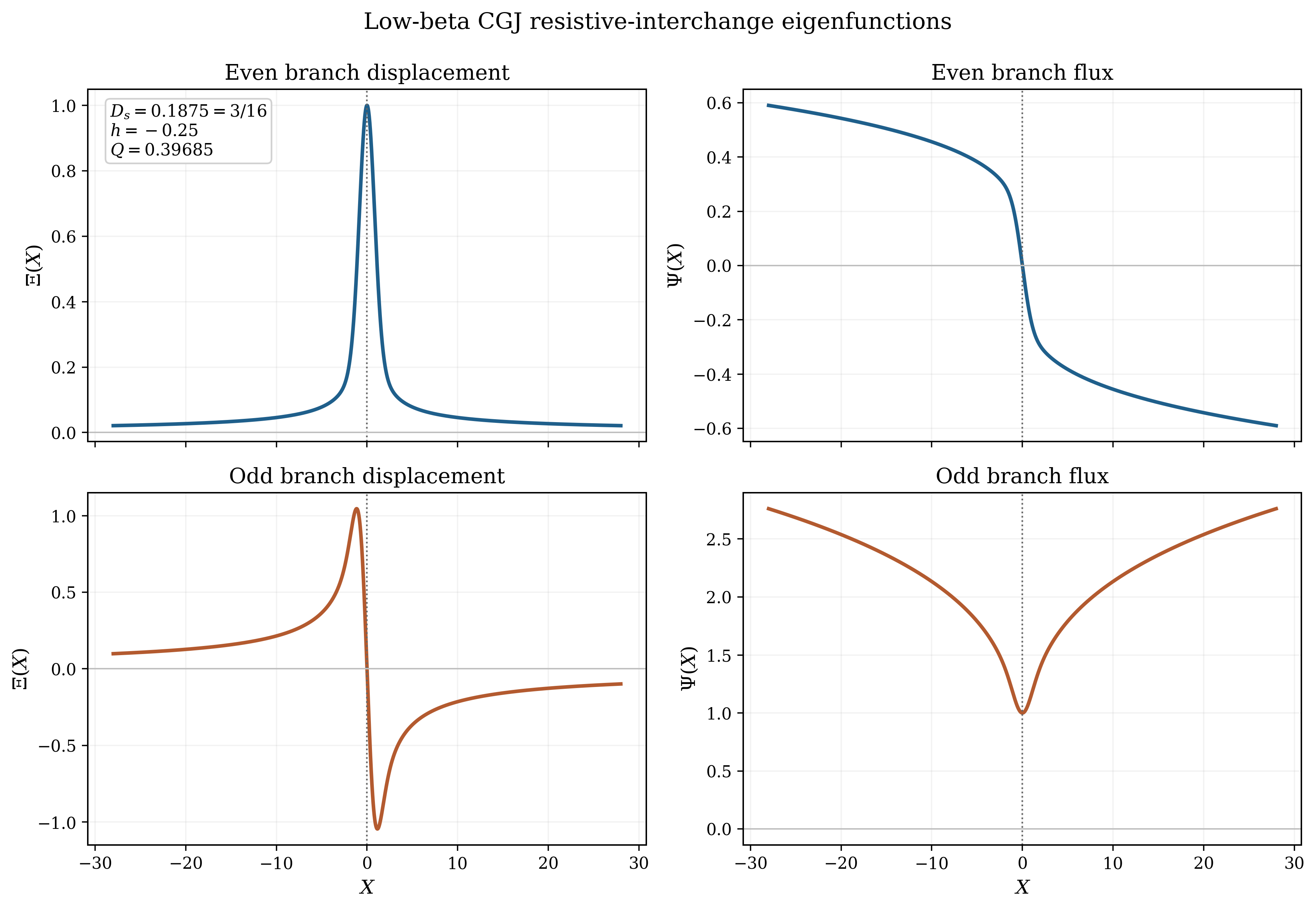
At \(D_s=3/16\), the low-\(\beta \) two-field problem gives the standard Coppi benchmark (28.39). Numerically, the even and
odd parity branches are then almost degenerate: both hit the same matched eigenvalue to within the
numerical accuracy of the finite domain and asymptotic fit. Figure 28.1 shows the corresponding parity
basis functions, while Fig. 28.2 shows the matching diagnostic used to recover the benchmark
\(Q\).
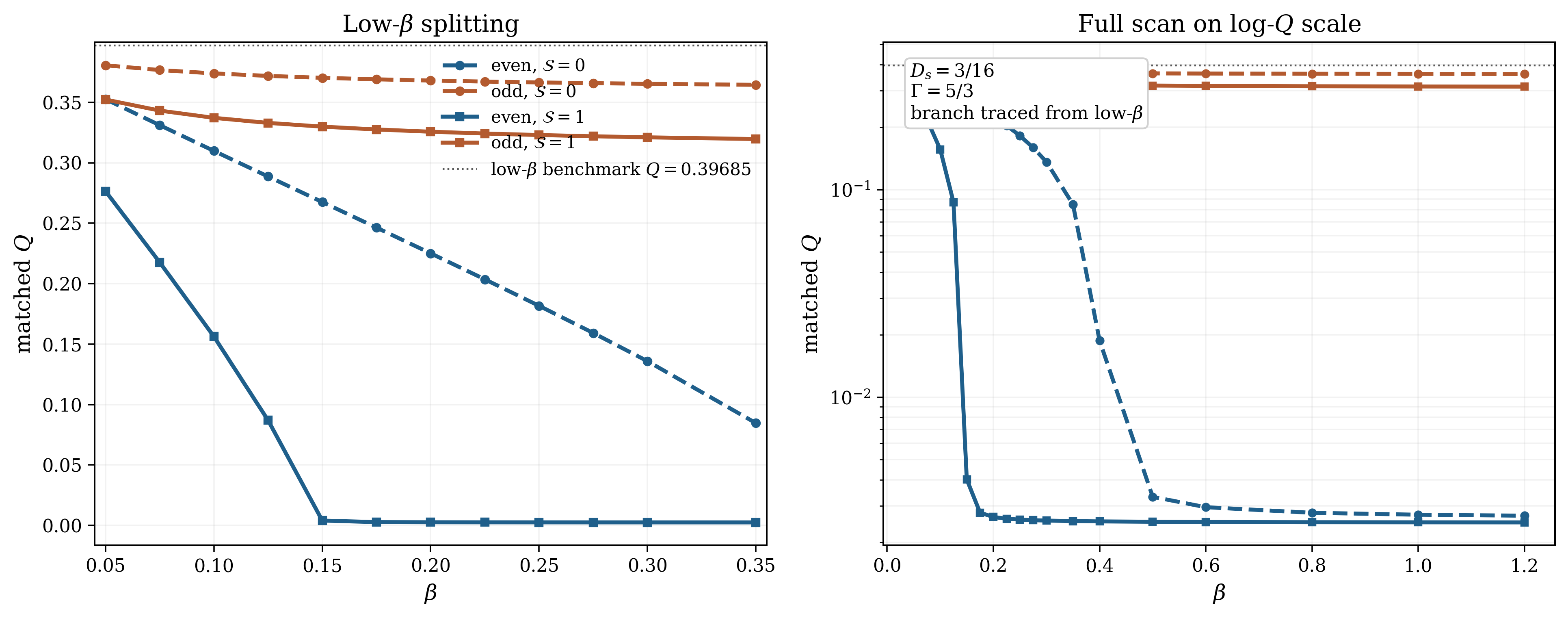
Finite-\(\beta \): the degeneracy is lifted.
Once the full three-field system (60)–(62) is retained, the even and odd branches separate. To compare like
with like, the \(\beta \)-scan shown below follows the high-\(Q\) continuation connected continuously to the low-\(\beta \) Coppi
branch. This avoids jumping to unrelated tiny-\(Q\) roots that can also appear in the full three-field
problem.
For the representative case
\[\Gamma =\frac 53, \qquad \beta =0.10, \qquad \Gamma \beta =\frac 16,\]
the matched roots are \[(Q_{\rm even},Q_{\rm odd})=(0.30978,0.37390) \qquad \text {for } \mathcal S=0,\]
whereas \[(Q_{\rm even},Q_{\rm odd})=(0.15627,0.33714) \qquad \text {for } \mathcal S=1.\]
Thus finite pressure breaks the low-\(\beta \) parity degeneracy, and the stabilizing geometric term \(\mathcal S\) pushes the even
branch downward much more strongly than the odd branch.
Which mode is most likely to grow?
Since the physical growth rate is \(\gamma = Q\gamma _R\), the larger positive value of \(Q\) is the faster-growing branch at fixed local
resistive-interchange scale \(\gamma _R\). Figure 28.3 therefore answers the question directly: the tearing-like odd branch
is the branch most likely to dominate once finite-\(\beta \) effects become important. It remains on an order-unity \(Q\)
branch, while the interchange-like even branch is pushed toward much smaller \(Q\), especially when
\(\mathcal S\sim 1\).
Why this is also the island-forming mode.
This dynamical dominance matters topologically because the odd branch is exactly the one with \(\Psi (0)\neq 0\). From
Eq. (28.32), \(\Psi \) is proportional to the radial magnetic perturbation \(b_r\), so finite \(\Psi (0)\) means finite \(b_r\) right in the layer.
The mode therefore reconnects field lines and produces a genuine magnetic island, just as in ordinary
tearing. By contrast, the even branch has \(\Psi (0)=0\) and is not island-forming at lowest order. So the same parity
branch that is numerically more robust at finite \(\beta \) is also the branch that produces observable
pressure-driven islands in a \(\Delta '\)-stable plasma.
29.5 How a negative \(\Delta '\) can still give islands
The outer ideal region is solved exactly as in the tearing lecture. One again obtains the logarithmic
matching index
\[\Delta ' = \left .\frac {\psi '}{\psi }\right |_{r_s^-}^{r_s^+}.\]
If \(D_s=0\), the tearing-parity branch collapses to the classical FKR problem and Eq. (27.59) is recovered. At
finite pressure gradient, however, (28.38) shows that the layer contains a second source of free
energy.
The key qualitative point.
For the tearing-like branch, the matching relation is no longer a pure \(\Delta '\leftrightarrow \gamma ^{5/4}\) FKR law. The pressure-gradient
term contributes a second, destabilizing part to the layer response. In Coppi’s language, that is why a
mode can remain unstable even when the classical outer tearing index would by itself predict stability
Coppi et al. (1966). Put differently, \(\Delta '\) is still part of the answer, but it is no longer the only place where the
free energy enters.
Why low shear helps this happen.
The same statement can be made with no formal dispersion relation at all. Since \(D_s\propto |p'|/[q']^2\), reducing the shear
makes the pressure term larger. Since the interchange drive sits inside the resistive layer, it is the
tearing-like parity that translates that drive into a finite \(\psi (0)\), and therefore into islands. That is the simplest
mathematical route from “buoyancy” to “reconnection.”
So is there a pressure-gradient threshold analogous to \(\Delta '\)?
There is a clean local onset parameter, but it is not \(p'\) by itself. In cylindrical form it is \(D_s\), because pressure
enters only in combination with curvature and magnetic shear: Eq. (28.2). With the sign conventions used
here, \(D_s>0\) means that the local pressure-curvature term is destabilizing, while the stronger ideal-Suydam
threshold is \(D_s>1/4\). So the transparent local resistive-interchange onset statement is precisely the window
already identified in Eq. (28.4): \[ 0<D_s<\frac 14. \] That is the closest pressure-gradient analogue of a one-number
threshold.
But it is not a replacement for \(\Delta '\). The two quantities answer different questions. \(\Delta '\) is an outer matching
index: it tells us how the ideal magnetic solution leans into the inner layer. \(D_s\) is an inner drive coefficient: it
tells us whether pressure and curvature can feed energy into that layer once the resonant geometry is
present. For the pure interchange-like branch, \(D_s>0\) is already the essential local instability condition. For the
tearing-like branch, however, island formation still depends on how that local drive couples to the
outer solution, so the onset is really a condition in the \((D_s,\Delta ')\) plane, not a single critical value of
\(p'\).
This is exactly what becomes more explicit in toroidal geometry. In the Glasser–Greene–Johnson
formulation the local quantity \(D_s\) is replaced by its toroidal counterpart \(D_R\). Pure resistive interchange is stable
when \(D_R<0\), but the tearing branch is not then determined by pressure alone: favorable curvature can instead
raise the threshold so that the outer matching parameter must exceed a critical value \(A_c\) (equivalently a
critical \(\Delta '_c\)) before the modified tearing mode becomes unstable.
29.6 A worked example: outer tearing stable, pressure driven inside
It is helpful to write one example all the way through. Reuse the current profile from the tearing lecture,
\[J_z(r)= \begin {cases} J_0, & 0<r<c,\\[4pt] 0, & c<r<a, \end {cases} \tag{28.51}\]
so that the outer \(m=2\) tearing index is given by Eq. (27.34). Add a smooth pressure profile, \[p(r)=p_0\left (1-\frac {r^2}{a^2}\right ), \qquad p'(r)=-\frac {2p_0 r}{a^2}. \tag{28.52}\]
In the current-free annulus of the step-current equilibrium, \[q(r)=q_c\frac {r^2}{c^2}, \qquad \frac {q'(r)}{q(r)}=\frac {2}{r}.\]
Substituting this into (28.2) gives \[D_s = -\frac {2\muo q_s^2}{r_s B_z^2 q_s'^2}\,p'(r_s) = -\frac {\muo r_s}{2B_z^2}p'(r_s) = \frac {\muo p_0}{B_z^2}\frac {r_s^2}{a^2}. \tag{28.54}\]
If we define a guide-field beta based on \(B_z\), \[\beta _z \equiv \frac {2\muo p_0}{B_z^2},\]
then \[D_s = \frac {\beta _z}{2}\frac {r_s^2}{a^2}. \tag{28.56}\]
Thus Suydam stability requires \[\frac {\beta _z}{2}\frac {r_s^2}{a^2}<\frac 14.\]
Now choose \[\frac {c}{a}=0.50, \qquad \frac {r_s}{a}=0.80, \qquad m=2, \qquad \beta _z=0.30. \tag{28.58}\]
Then \[D_s = \frac {0.30}{2}(0.80)^2 = 0.096 < \frac 14,\]
so the surface is ideally Suydam-stable.
At the same time, the tearing lecture gives
\[x\equiv \frac {c}{r_s}=0.625, \qquad y\equiv \frac {a}{r_s}=1.25,\]
and therefore, from Eq. (27.34), \[\Delta ' = \frac {4}{r_s} \frac {2x^2y^4-x^4-y^4}{(1-x^2)^2(y^4-1)} \approx -\frac {6.41}{a} < 0. \tag{28.61}\]
So the outer current profile by itself is tearing stable, while the local ideal problem is also stable.
Nevertheless \(D_s>0\), and because the tearing-like parity has \(\Psi (0)\neq 0\), the pressure gradient can still drive an
island-forming resistive branch. This is exactly the regime in which the lecture earns its keep: a \(\Delta '\)-stable
plasma can still reconnect because the free energy is no longer purely magnetic.
Make the instability explicit.
For this particular choice the local shear length is
\[L_s = \left |\frac {q_s}{q_s'}\right | = \frac {r_s}{2} = 0.40\,a, \qquad k_\perp = \frac {m}{r_s} = \frac {2.5}{a}. \tag{28.62}\]
Hence the characteristic resistive-interchange rate from Eq. (28.15) is \[\gamma _R = \left (\eta _m\frac {k_\perp ^2 V_A^2}{L_s^2}\right )^{1/3} = \left (39.1\,\frac {\eta _m V_A^2}{a^4}\right )^{1/3}. \tag{28.63}\]
To keep the worked example analytic, use the transparent local estimate \[\gamma _{\rm RI} \sim D_s^{1/3}\gamma _R . \tag{28.64}\]
An exact prefactor requires solving the parity-selected inner problem (60)–(62) and imposing the matching
condition (28.41). The estimate only fixes the natural positive growth scale. For the present surface, \(D_s=0.096\),
\[\gamma _{\rm RI} \sim (0.096)^{1/3}\gamma _R \approx 0.46\,\gamma _R \approx 1.57\left (\frac {\eta _m V_A^2}{a^4}\right )^{1/3} >0.\]
So this equilibrium is not merely “Suydam stable” and “\(\Delta '\)-stable.” It still has a positive resistive-interchange
growth rate. Because the branch we are following has tearing parity, \(\psi (r_s,t)\) is finite and grows like
\[\psi (r_s,t)\propto e^{\gamma _{\rm RI} t},\]
which means that the island half-width from Eq. (27.67) grows as \[w(t)\propto |\psi (r_s,t)|^{1/2}\propto e^{\gamma _{\rm RI} t/2}. \tag{28.67}\]
That is the last logical step the example needs: the mode is outer tearing stable, locally ideal
stable, and still island-forming because the pressure-gradient drive lives inside the resistive
layer.
What this example teaches.
The example is intentionally simple, but the logic is robust.
-
1.
- The sign of \(\Delta '\) is controlled mainly by the current profile and the exterior solution.
-
2.
- The sign and size of \(D_s\) are controlled by the pressure gradient and the magnetic shear.
-
3.
- A positive local resistive-interchange root \(\gamma _{\rm RI}>0\) with tearing parity turns pressure drive into actual
island growth, \(w\propto e^{\gamma _{\rm RI} t/2}\), rather than into purely convective flute motion.
That separation of roles is physically useful, and it is the main reason this lecture sits naturally near the
tearing lecture.
A toroidal caution.
This lecture is intentionally cylindrical, so the local ideal criterion here is Suydam, not Mercier. In a
tokamak, Mercier replaces Suydam on the ideal side, while the resistive layer is described by
the toroidal Glasser–Greene–Johnson generalization. The important lesson is that ideal local
stability and resistive-layer stability are related but not identical: Mercier stability removes the
immediate ideal catastrophe, but it does not by itself eliminate pressure-driven resistive layer
physics.
29.7 Experimental Perspective: flux pumping and hybrid operation
The cylindrical analysis is not yet a tokamak hybrid
discharge ,
but it already contains the seed of that story. A low-shear core with \(q\approx 1\) is exactly the place where a
pressure-driven \((m,n)=(1,1)\) mode can compete with the ordinary internal kink. In modern toroidal language, one often
calls that saturated, low-shear branch a quasi-interchange mode.
Jardin’s flux-pumping picture.
Three-dimensional resistive-MHD simulations by Jardin, Ferraro, and Krebs found stationary helical core
states in which a saturated central interchange-like mode drives a near-helical flow and an effective
dynamo loop voltage, thereby keeping the central safety factor close to unity rather than letting it
fall into ordinary sawtoothing Jardin et al. (2015). The more detailed follow-on analysis of
Krebs et al. showed that, in hybrid-like conditions, the dominant nonlinear mechanism is a
saturated \((m,n)=(1,1)\) quasi-interchange instability that generates an effective negative loop voltage in the
plasma center Krebs et al. (2017). Jardin, Krebs, and Ferraro later recast that same idea as a
candidate explanation of the longstanding sawtooth problem in auxiliary-heated tokamaks Jardin
et al. (2020).
Why the hybrid scenario is the natural home for this physics.
The JET hybrid scenario was explicitly developed as an ITER-relevant mode of operation with \(q_0\) or
\(q_{\min }\) near unity, low central shear, long pulse duration, and improved stability margins Joffrin
et al. (2005). DIII-D later emphasized that high-\(\beta _N\) hybrid operation is attractive for ITER and FNSF
steady-state missions, precisely because the current profile can be kept broad while avoiding
deleterious core activity Turco et al. (2015). More recently, ASDEX Upgrade reported direct
experimental evidence of magnetic flux pumping in a sawtooth-free hybrid scenario, with the
central safety factor clamped close to unity by anomalous current redistribution Burckhart
et al. (2023).
What survives from the cylindrical lecture.
The full tokamak problem is toroidal, nonlinear, and three-dimensional; it contains bootstrap current,
heating and current-drive source terms, toroidal coupling, and real transport. But the simple
cylindrical lecture still teaches the central analytic lesson: in a low-shear core, a pressure-driven
resistive mode can have either convective or island-forming parity, and the latter provides a
clean route to current redistribution. That is why this old pinch problem still feels surprisingly
modern.
Takeaways
- The relevant cylindrical resistive-interchange window is \(0<D_s<1/4\): pressure drive is present,
but ideal Suydam instability has not yet appeared.
- In toroidal geometry Suydam is replaced on the ideal side by Mercier, but ideal
local stability still does not by itself settle the resistive-layer problem.
- Low magnetic shear matters because \(D_s\propto |p'|/[q']^2\).
- The inner resistive problem has two parity classes. The interchange-like branch has
\(\Psi (0)=0\); the tearing-like branch has \(\Psi (0)\neq 0\) and therefore forms islands.
- A negative classical tearing index \(\Delta '\) does not guarantee stability once
pressure-gradient drive is allowed to enter the layer.
- The modern flux-pumping / hybrid-scenario story is the toroidal, nonlinear
descendant of the same low-shear pressure-driven physics.
Bibliography
Walter M. Elsasser. Hydromagnetic dynamo theory. Reviews of Modern Physics, 28(2):135–163, 1956. doi:10.1103/RevModPhys.28.135.
L. Woltjer. A theorem on force-free magnetic fields. Proceedings of the National Academy of Sciences of the United States of America, 44(6):489–491, 1958a. doi:10.1073/pnas.44.6.489.
L. Woltjer. On hydromagnetic equilibrium. Proceedings of the National Academy of Sciences of the United States of America, 44(9):833–841, 1958b. doi:10.1073/pnas.44.9.833.
Martin D. Kruskal and Russell M. Kulsrud. Equilibrium of a magnetically confined plasma in a toroid. Physics of Fluids, 1(4):265–274, 1958. doi:10.1063/1.1705884.
J. B. Taylor. Relaxation of toroidal plasma and generation of reverse magnetic fields. Physical Review Letters, 33(19):1139–1141, 1974. doi:10.1103/PhysRevLett.33.1139.
S. C. Prager. Transport and fluctuations in reversed field pinches. Plasma Physics and Controlled Fusion, 32(11):903–916, 1990. doi:10.1088/0741-3335/32/11/006.
Sergio Ortolani and Dalton D. Schnack. Magnetohydrodynamics of Plasma Relaxation. World Scientific, Singapore, 1993. ISBN 9789810208608. doi:10.1142/1564.
T. R. Jarboe. Review of spheromak research. Plasma Physics and Controlled Fusion, 36(6):945–990, 1994. doi:10.1088/0741-3335/36/6/002.
T. H. Jensen and M. S. Chu. Current drive and helicity injection. Physics of Fluids, 27(12):2881–2885, 1984. doi:10.1063/1.864602.
A. H. Boozer. Helicity content and tokamak applications of helicity. Physics of Fluids, 29(12):4123–4130, 1986. doi:10.1063/1.865756.
S. C. Jardin, N. Ferraro, and I. Krebs. Self-organized stationary states of tokamaks. Physical Review Letters, 115(21):215001, 2015. doi:10.1103/PhysRevLett.115.215001.
I. Krebs, S. C. Jardin, S. Günter, K. Lackner, M. Hölzl, E. Strumberger, and N. Ferraro. Magnetic flux pumping in 3d nonlinear magnetohydrodynamic simulations. Physics of Plasmas, 24(10):102511, 2017. doi:10.1063/1.4990704.
S. C. Jardin, I. Krebs, and N. Ferraro. A new explanation of the sawtooth phenomena in tokamaks. Physics of Plasmas, 27(3):032509, 2020. doi:10.1063/1.5140968.
H. Ji, A. F. Almagri, S. C. Prager, and J. S. Sarff. Time-resolved observation of discrete and continuous magnetohydrodynamic dynamo in the reversed-field pinch edge. Physical Review Letters, 73(5):668–671, 1994. doi:10.1103/PhysRevLett.73.668.
H. Ji and S. C. Prager. The $ $ dynamo effects in laboratory plasmas. Magnetohydrodynamics, 38(1-2):191–210, 2002. doi:10.22364/mhd.38.1-2.15.
R. H. Cameron, M. Dikpati, and A. Brandenburg. The global solar dynamo. Space Science Reviews, 210:367–395, 2017. doi:10.1007/s11214-015-0230-3.
C. G. Gimblett and M. L. Watkins. MHD turbulence theory and its implications for the reversed field pinch. In Proceedings of the 7th European Conference on Controlled Fusion and Plasma Physics, volume 1, page 103, Geneva, 1975. European Physical Society. Lausanne, Switzerland.
Zensho Yoshida. Roles of magnetic helicity in plasma confinement. Journal of Nuclear Science and Technology, 27(3):193–204, 1990. doi:10.3327/jnst.27.193.
M. Ono, G. J. Greene, D. S. Darrow, C. B. Forest, H. K. Park, and T. H. Stix. Steady-state tokamak discharge via dc helicity injection. Physical Review Letters, 59(19):2165–2168, 1987. doi:10.1103/PhysRevLett.59.2165.
D. S. Darrow, M. Ono, C. B. Forest, G. J. Greene, Y. S. Hwang, H. K. Park, R. J. Taylor, P. A. Pribyl, J. D. Evans, K. F. Lai, and J. R. Liberati. Properties of dc helicity injected tokamak plasmas. Physics of Fluids B: Plasma Physics, 2(6):1415–1420, 1990. doi:10.1063/1.859573.
R. Raman and V. F. Shevchenko. Solenoid-free plasma start-up in spherical tokamaks. Plasma Physics and Controlled Fusion, 56(10):103001, 2014. doi:10.1088/0741-3335/56/10/103001.
C. B. Forest, Y. S. Hwang, M. Ono, and D. S. Darrow. Internally generated currents in a small-aspect-ratio tokamak geometry. Physical Review Letters, 68(24):3559–3562, 1992. doi:10.1103/PhysRevLett.68.3559.
Y. S. Hwang, C. B. Forest, D. S. Darrow, G. J. Greene, and M. Ono. Reconstruction of current density distributions in the cdx-u tokamak. Review of Scientific Instruments, 63(10):4747–4749, 1992. doi:10.1063/1.1143628.
D. J. Battaglia, M. W. Bongard, R. J. Fonck, and A. J. Redd. Tokamak startup using outboard current injection on the pegasus toroidal experiment. Nuclear Fusion, 51(7):073029, 2011. doi:10.1088/0029-5515/51/7/073029.
K. Kuroda, R. Raman, T. Onchi, M. Hasegawa, K. Hanada, M. Ono, B. A. Nelson, J. Rogers, R. Ikezoe, H. Idei, T. Ido, M. Nagata, O. Mitarai, N. Nishino, Y. Otsuka, Y. Zhang, K. Kono, S. Kawasaki, T. Nagata, A. Higashijima, et al. Demonstration of transient CHI startup using a floating biased electrode configuration. Nuclear Fusion, 64(1):014002, 2024. doi:10.1088/1741-4326/ad0dd6.
T. Shinya, Y. Takase, T. Wakatsuki, A. Ejiri, H. Furui, J. Hiratsuka, K. Imamura, T. Inada, H. Kakuda, H. Kasahara, R. Kumazawa, C. Moeller, T. Mutoh, Y. Nagashima, K. Nakamura, A. Nakanishi, T. Oosako, K. Saito, T. Seki, M. Sonehara, H. Togashi, S. Tsuda, N. Tsujii, and T. Yamaguchi. Non-inductive plasma start-up experiments on the TST-2 spherical tokamak using waves in the lower-hybrid frequency range. Nuclear Fusion, 55(7):073003, 2015. doi:10.1088/0029-5515/55/7/073003.
M. Inomoto, T. G. Watanabe, K. Gi, K. Yamasaki, S. Kamio, R. Imazawa, R. Hihara, A. Kuwahata, Y. Ono, H. Tanabe, T. Kanki, O. Mitarai, T. Hayashi, T. Umeda, M. Stoneking, and R. Kulsrud. Centre-solenoid-free merging start-up of spherical tokamak plasmas in UTST. Nuclear Fusion, 55(3):033013, 2015. doi:10.1088/0029-5515/55/3/033013.
P. M. Bellan. Physical model of current drive by ac helicity injection. Physics of Fluids, 27(8):2191–2192, 1984. doi:10.1063/1.864846.
P. M. Bellan. Mode-beating model of ac helicity injection. Physical Review Letters, 54(13):1381–1384, 1985. doi:10.1103/PhysRevLett.54.1381.
S. Yamaguchi, M. Schaffer, and Y. Kondoh. Preliminary oscillating fluxes current drive experiment in diii-d tokamak. Fusion Engineering and Design, 26(1–4):121–132, 1995. doi:10.1016/0920-3796(94)00177-9.
K F Schoenberg, J C Ingraham, C P Munson, P G Weber, D A Baker, R F Gribble, R B Howell, G Miller, W A Reass, A E Schofield, S Shinohara, and G A Wurden. Oscillating field current drive experiments in a reversed field pinch. The Physics of Fluids, 31(8):2285–2291, 1988. doi:10.1063/1.866629.
K. J. McCollam, A. P. Blair, S. C. Prager, and J. S. Sarff. Oscillating-field current-drive experiments in a reversed field pinch. Physical Review Letters, 96(3):035003, 2005. doi:10.1103/physrevlett.96.035003.
A. Burckhart, A. Bock, R. Fischer, T. Pütterich, J. Stober, S. Günter, A. Gude, J. Hobirk, M. Hölzl, V. Igochine, I. Krebs, M. Maraschek, M. Reisner, and the ASDEX Upgrade Team. Experimental evidence of magnetic flux pumping in ASDEX upgrade. Nuclear Fusion, 63(12):126056, 2023. doi:10.1088/1741-4326/ad067b.
J Stober, A C C Sips, C Angioni, C B Forest, O Gruber, J Hobirk, L D Horton, C F Maggi, M Maraschek, P Martin, P J Mc Carthy, V Mertens, Y S Na, M Reich, A Stäbler, G Tardini, and H Zohm. The role of the current profile in the improved h-mode scenario in ASDEX upgrade. Nuclear Fusion, 47(8):728–737, 2007. ISSN 0029-5515. doi:10.1088/0029-5515/47/8/002.
Francesca Turco, Clinton C. Petty, Timothy C. Luce, Thomas N. Carlstrom, Michael A. Van Zeeland, William Heidbrink, Francesco Carpanese, Wayne M. Solomon, Christopher T. Holcomb, and John R. Ferron. The high-$ _N$ hybrid scenario for ITER and FNSF steady-state missions. Physics of Plasmas, 22(5):056113, 2015. doi:10.1063/1.4921161.
Harold P. Furth, John Killeen, and Marshall N. Rosenbluth. Finite-resistivity instabilities of a sheet pinch. Physics of Fluids, 6(4):459–484, 1963. doi:10.1063/1.1706761.
Bruno Coppi, John M. Greene, and John L. Johnson. Resistive instabilities in a diffuse linear pinch. Nuclear Fusion, 6(2):101–117, 1966. doi:10.1088/0029-5515/6/2/003.
E. Joffrin, A. C. C. Sips, J. F. Artaud, A. Bécoulet, L. Bertalot, R. Budny, P. Buratti, P. Belo, C. D. Challis, F. Crisanti, M. De Baar, P. de Vries, C. Gormezano, C. Giroud, O. Gruber, G. T. A. Huysmans, F. Imbeaux, A. Isayama, X. Litaudon, P. J. Lomas, D. C. McDonald, Y. S. Na, S. D. Pinches, A. Staebler, T. Tala, A. Tuccillo, K. D. Zastrow, and JET-EFDA Contributors. The `hybrid' scenario in JET: Towards its validation for ITER. Nuclear Fusion, 45(7):626–634, 2005. doi:10.1088/0029-5515/45/7/010.
Problems
-
Problem 29.1.
- Starting from Eq. (28.2), derive Eq. (28.54) for the parabolic pressure profile
(28.52).
-
Problem 29.2.
- For the numerical choice (28.58), verify explicitly that \(D_s<1/4\) while Eq. (28.61) gives \(\Delta '<0\).
-
Problem 29.3.
- Show directly from Eqs. (60)–(62) that \(\Psi \) must have the opposite parity to \(\Xi \) and \(\Upsilon \).
-
Problem 29.4.
- Using Eq. (28.15), estimate how the resistive-interchange growth rate changes
if the magnetic shear is reduced by a factor of two while all other equilibrium
quantities are held fixed.
-
Problem 29.5.
- Explain in words why the tearing-like parity is the one relevant for flux-pumping
and current-redistribution discussions in low-shear hybrid plasmas.