Lecture 20
The Kruskal–Shafranov Kink Mode
Overview
This lecture is one of the canonical current-driven stability problems in MHD. It
has four jobs:
-
1.
- derive the external kink in the surface-current model carefully enough that the
Kruskal–Shafranov threshold is unmistakable;
-
2.
- show how an ideal conducting wall changes the vacuum matching and why the
periodic problem develops the familiar but somewhat misleading two-root structure;
-
3.
- explain how a resistive wall mode is just the slow return of a kink that was stabilized
only by wall currents; and
-
4.
- treat the finite-length, line-tied column explicitly, including the important ideal-wall
threshold \[ q_a < 1-\frac {a^2}{b^2}, \] which is different from the periodic result.
The current-driven kink is the place where several themes of these notes finally meet: the energy principle
of Lecture 13, vacuum matching, the meaning of the safety factor, and the role of conducting boundaries.
It is also one of the problems where a seemingly small choice of boundary condition — periodic versus line
tied — changes the answer in an instructive way. That is why the Kruskal–Shafranov problem remained
“classic” for so long: it is simple enough to solve analytically, but subtle enough to keep revealing
something new.
Historical Perspective
The first clean surface-current demonstration of the current-driven kink was the
Kruskal–Schwarzschild analysis of the \(Z\) pinch Kruskal and Schwarzschild (1954).
Kruskal’s later treatment with axial field, together with Shafranov’s contemporaneous
work, turned that result into the screw-pinch stability limit now summarized as the
Kruskal–Shafranov criterion Kruskal and Tuck (1958); Shafranov (1957, 1970). Much
later, it was realized that the finite-length line-tied problem is not captured correctly
by simply setting \(k=2\pi /L\). The missing ingredient is that the exact line-tied eigenfunction must
satisfy end-plate boundary conditions, and that forces one to mix more than one axial
harmonic. That correction is not a minor technicality: it changes the stability threshold.
20.1 The surface-current model and the periodic Kruskal–Shafranov limit
The cleanest derivation starts from the same hollow-current equilibrium used in the classic papers. The
plasma occupies \(r<a\). Inside the plasma the field is taken to be purely axial,
\[\B _{\rm pl} = B_z\,\vect {e}_z,\]
while outside the plasma the vacuum field is \[\B _{\rm vac} = B_z\,\vect {e}_z + B_\theta (r)\,\vect {e}_\theta , \qquad B_\theta (r)=B_\theta (a)\frac {a}{r}. \tag{20.2}\]
The jump in tangential magnetic field corresponds to a surface current, \[\muo \vect {K} = \hat {\vect {n}}\times \left (\B _{\rm vac}-\B _{\rm pl}\right ),\]
so the discontinuity in \(B_\theta \) is an axial sheet current, \[K_z = \frac {B_\theta (a)}{\muo }.\]
Equilibrium across the interface.
In static equilibrium, the normal stress must be continuous across the plasma–vacuum boundary. With
isotropic pressure this gives
\[\left [p+\frac {B^2}{2\muo }\right ]=0. \tag{20.5}\]
If we choose the inside and outside axial fields to be equal, \[B_{z,\rm in}=B_{z,\rm out}=B_z,\]
then (20.5) reduces to \[\boxed { p = \frac {B_\theta ^2(a)}{2\muo }. } \tag{20.7}\]
This is the standard hollow-current surface-current equilibrium: the plasma pressure is held in by the
external poloidal field generated by the axial sheet current.
Boundary condition on the perturbed radial field.
From the frozen-in relation for the perturbed magnetic field,
\[\B _1 = \curl (\vect {\xi }\times \B _0), \tag{20.8}\]
which was derived in Lecture 13 as (13.3), one can impose that the perturbed field remain tangent to the
perturbed surface. Write the displaced boundary as \[F(r,\theta ,z)=r-a-\xi _r(\theta ,z)=0.\]
To first order, \[\grad F = \vect {e}_r -\frac {1}{a}\pp {\xi _r}{\theta }\vect {e}_\theta -\pp {\xi _r}{z}\vect {e}_z.\]
Because \[\begin{aligned}(\B _0+\B _1)\cdot \grad F & =0 \\ & = \delta B_r - \frac {B_\theta }{a}\pp {\xi _r}{\theta } - B_z\pp {\xi _r}{z}.\end{aligned}\]
on the perturbed surface and \(B_{0r}=0\), the linearized boundary condition is
\[\delta B_r =i m \frac {B_\theta }{a} +i k B_z\]
For a helical normal mode, \[\xi _r = \xi _0 e^{i(m\theta +kz)},\]
this becomes \[\boxed { \delta B_r = i\left (\frac {mB_\theta (a)}{a}+kB_z\right ) \xi _0 e^{i(m\theta +kz)}. } \tag{20.15}\]
This single interface relation is the place where the field-line pitch enters the calculation.
Vacuum solution outside the plasma.
In the vacuum region the perturbed field is curl free and divergence free, so we write
\[\delta \B = \grad \Phi , \qquad \nabla ^2 \Phi = 0.\]
Tutorial
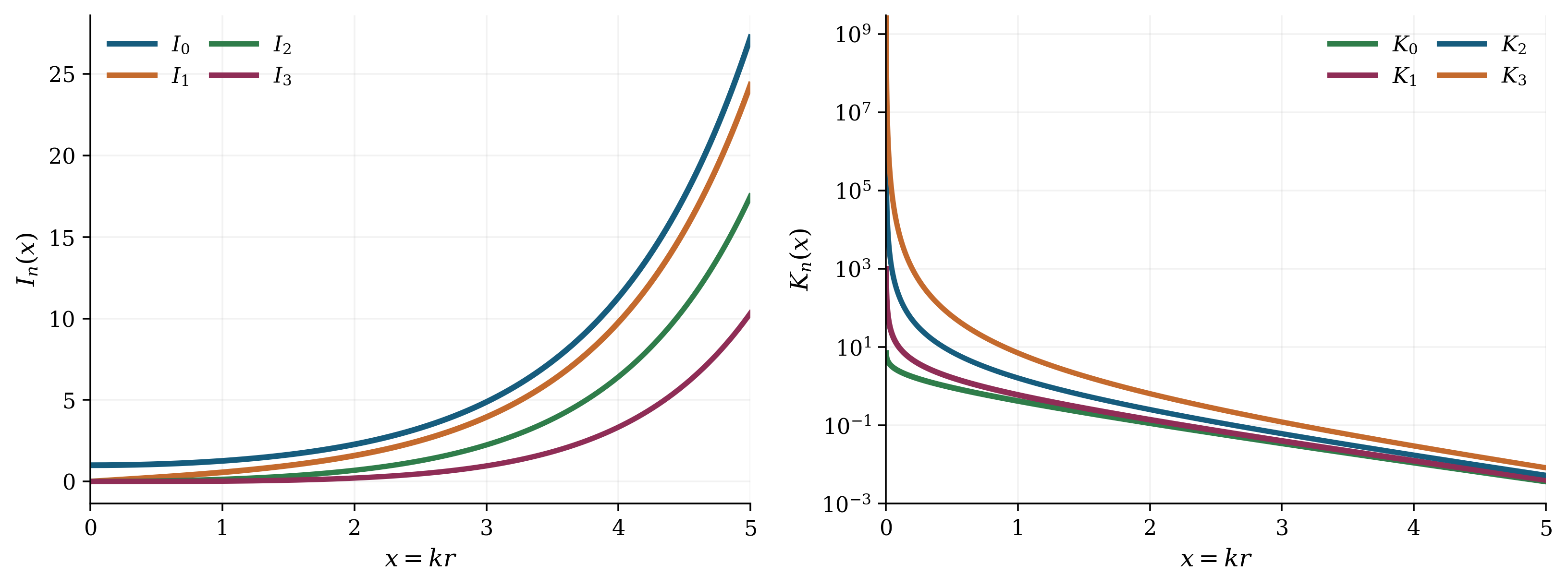
Tutorial: why modified Bessel functions appear in the vacuum field. In vacuum there
is no perturbed current, so \[ \nabla \times \delta \B =0, \qquad \nabla \cdot \delta \B =0. \] That is why we can write \(\delta \B =\grad \Phi \) with \(\nabla ^2\Phi =0\). If we separate variables as \[ \Phi (r,\theta ,z)=\phi _m(r)e^{i(m\theta +kz)}, \] then
the radial function satisfies \[ \frac {d^2\phi _m}{dr^2} +\frac {1}{r}\frac {d\phi _m}{dr} -\left (\frac {m^2}{r^2}+k^2\right )\phi _m=0. \] With \(x\equiv |k|r\), this becomes \[ x^2\phi _m''+x\phi _m'-(x^2+m^2)\phi _m=0, \] which is the modified Bessel equation.
Its two independent solutions are \[ \phi _m(x)=A I_m(x)+C K_m(x). \] The geometry decides which one is physical:
- \(I_m\) is regular at \(r=0\), so it is the acceptable solution near the axis;
- \(K_m\) decays as \(r\to \infty \), so it is the acceptable solution in an unbounded exterior vacuum;
- in a vacuum annulus \(a<r<b\), one keeps both \(I_m\) and \(K_m\), then uses the wall condition to fix their
combination.
Because \(\delta \B =\grad \Phi \), the matching condition on the radial field involves \(I_m'\) and \(K_m'\), not just \(I_m\) and \(K_m\) themselves.
In the long-wavelength limit \(|k|r\ll 1\) these reduce to the familiar harmonic-cylinder behaviors, \[ I_m(|k|r)\propto r^m, \qquad K_m(|k|r)\propto r^{-m}\quad (m\ge 1), \] while \(K_0(|k|r)\sim -\ln (|k|r)\).
Thus for \(m=1\) one recovers the simple form \(\Phi \sim Ar+C/r\). Figure 20.2 makes the roles visually obvious: \(I_n\) stays
finite at the axis and grows outward, whereas \(K_n\) decays outward and is singular at the axis for
\(n\ge 1\).
For a mode \(e^{i(m\theta +kz)}\) that decays as \(r\to \infty \),
\[\Phi = A K_m(|k|r)e^{i(m\theta +kz)},\]
with \(K_m\) the modified Bessel function of the second kind. Therefore \[\delta B_r^{\rm vac} = A|k|K_m'(|k|r)e^{i(m\theta +kz)}.\]
Matching to (20.15) at \(r=a\) gives \[A = \frac {i\left (\frac {mB_\theta (a)}{a}+kB_z\right )\xi _0}{|k|K_m'(|k|a)}. \tag{20.19}\]
Plasma term.
For \(m=1\) the plasma core moves almost rigidly, so the only important interior term is axial-field bending. Using
(13.3), repeated here
\[\begin{aligned}\delta W_P = \frac 12\int _P dV\Bigg [ & \underbrace {\frac {|\vect {Q}_\perp |^2}{\muo }}_{\text {field-line bending}} + \underbrace {\frac {B^2}{\muo } \left |\divergence \vect {\xi }_\perp + 2\,\vect {\xi }_\perp \cdot \vect {\kappa }\right |^2}_{\text {magnetic compression}} + \underbrace {\gamma p\,|\divergence \vect {\xi }|^2}_{\text {plasma compression}} \nonumber \\[0.5em] & - \underbrace {2\,(\vect {\xi }_\perp \cdot \grad p) (\vect {\xi }_\perp ^{*}\cdot \vect {\kappa })}_{\text {pressure--curvature coupling}} - \underbrace {\frac {J_\parallel }{B} (\vect {\xi }_\perp ^{*}\times \B )\cdot \vect {Q}_\perp }_{\text {current-driven term}} \Bigg ].\end{aligned}\]
with \(\B _0=B_z\vect {e}_z\),
\[\delta \B _{\rm pl} = \curl (\vect {\xi }\times B_z\vect {e}_z), \qquad |\delta \B _{\rm pl}|^2 = k^2 B_z^2 |\xi _0|^2,\]
which gives \[\boxed { \delta W_{\rm pl} = \frac {\pi a^2L}{2\muo }k^2B_z^2|\xi _0|^2. } \tag{20.22}\]
Surface Term.
From the surface term in the energy principle of Lecture 13, the interface contribution is
\[\delta W_{\rm surf} = \frac {1}{2}\int _{r=a} \xi _r^2 \left [\!\left [ \dd {}{r} \left ( p+\frac {B^2}{2\muo } \right ) \right ]\!\right ]dS.\]
Because the pressure is constant inside and outside in this simple model, only \(B_\theta (r)\) contributes. Using (20.2),
\[\dd {}{r}\left (\frac {B_\theta ^2}{2\muo }\right ) = -\frac {B_\theta ^2(a)}{\muo a} \qquad (r=a),\]
so \[\boxed { \delta W_{\rm surf} = -\frac {\pi L}{2\muo }B_\theta ^2(a)|\xi _0|^2. } \tag{20.25}\]
Vacuum magnetic energy.
The vacuum contribution to the potential energy is
\[\delta W_{\rm vac} = \frac {1}{2\muo }\int _{\rm vac}|\delta \B |^2\,dV.\]
Since \(\delta \B =\grad \Phi \) and \(\nabla ^2\Phi =0\), Green’s identity \[\begin{aligned}\int _V \nabla \cdot (\Phi \nabla \Phi ) dV & = \int _V (\nabla \Phi )^2 dV + \int \Phi \cancelto {0}{\nabla ^2 \Phi } dV \\ \therefore \int _V (\nabla \Phi )^2 dV & = \int _S \Phi \nabla \Phi \cdot d \vect {S} \\\end{aligned}\]
reduces the volume integral to a boundary term,
\[\delta W_{\rm vac} = -\frac {1}{4\muo }\int _{r=a} \Phi ^*\,\delta B_r^{\rm vac}\,dS,\]
where the minus sign comes from the outward normal of the vacuum region at the plasma surface.
Carrying out the surface integral yields \[\boxed { \delta W_{\rm vac} = \frac {\pi aL}{2\muo } \Lambda _m(x) \left (\frac {mB_\theta (a)}{a}+kB_z\right )^2 |\xi _0|^2, } \tag{20.31}\]
with \[x\equiv |k|a, \qquad \Lambda _m(x)\equiv -\frac {K_m(x)}{|k|K_m'(x)}>0.\]
The least stable case is \(m=1\), so from this point onward we restrict attention to the external kink.
Total energy and the Kruskal–Shafranov threshold.
The total potential energy is the sum of the three pieces,
\[\delta W = \delta W_{\rm pl}+\delta W_{\rm surf}+\delta W_{\rm vac}.\]
Using (20.31), (20.25), and (20.22), \[\boxed { \delta W = \frac {\pi L}{2\muo }|\xi _0|^2 \left [ a^2k^2B_z^2 -B_\theta ^2(a) +a\Lambda _1(x) \left (kB_z+\frac {B_\theta (a)}{a}\right )^2 \right ]. } \tag{20.34}\]
In the long-wavelength limit \(|k|a\ll 1\), \[K_1(x)\sim \frac {1}{x}, \qquad K_1'(x)\sim -\frac {1}{x^2}, \qquad \Lambda _1(x)\to a.\]
Then (20.34) becomes \[\begin{aligned}\delta W &\to \frac {\pi L}{2\muo }|\xi _0|^2 \left [ a^2k^2B_z^2 -B_\theta ^2(a) +a^2\left (kB_z+\frac {B_\theta (a)}{a}\right )^2 \right ] \\ &= \frac {\pi a^2Lk^2B_z^2}{\muo }|\xi _0|^2 \left (1-\frac {1}{q_a}\right ),\end{aligned} \tag{20.37}\]
where for the unstable helicity we define
\[q_a \equiv \frac {2\pi a B_z}{L|B_\theta (a)|}, \qquad |k|=\frac {2\pi }{L}. \tag{20.38}\]
Therefore the periodic surface-current column is marginal at \[\boxed {q_a=1,} \tag{20.39}\]
and unstable for \(q_a<1\).
20.2 An ideal conducting wall in the periodic problem
Now place a perfectly conducting cylindrical wall at \(r=b>a\). The plasma and surface terms, (20.25) and (20.22),
do not change. Only the vacuum matching changes because the radial field must vanish at the
wall.
Vacuum field in the annulus \(a<r<b\).
In the vacuum annulus,
\[\delta \B =\grad \Phi , \qquad \nabla ^2\Phi =0,\]
and the general \(m=1\) solution is \[\Phi (r,\theta ,z) = \left [A I_1(\kappa r)+C K_1(\kappa r)\right ]e^{i(\theta +kz)}, \qquad \kappa \equiv |k|.\]
Hence \[\delta B_r^{\rm vac} = \kappa \left [A I_1'(\kappa r)+C K_1'(\kappa r)\right ]e^{i(\theta +kz)}.\]
The ideal-wall condition is \[\delta B_r^{\rm vac}(b)=0,\]
so \[A I_1'(\kappa b)+C K_1'(\kappa b)=0.\]
At the plasma boundary, \[\kappa \left [A I_1'(\kappa a)+C K_1'(\kappa a)\right ] = i\left (kB_z+\frac {B_\theta (a)}{a}\right )\xi _0.\]
It is convenient to define \[\alpha _b\equiv \frac {I_1'(\kappa b)}{K_1'(\kappa b)}, \qquad C=-\alpha _b A.\]
Then \[A = \frac {i\left (kB_z+\frac {B_\theta (a)}{a}\right )\xi _0}{\kappa \left [I_1'(\kappa a)-\alpha _b K_1'(\kappa a)\right ]},\]
and therefore \[\Phi (a) = \frac {i\left (kB_z+\frac {B_\theta (a)}{a}\right )\xi _0}{\kappa } \frac {I_1(\kappa a)-\alpha _b K_1(\kappa a)}{I_1'(\kappa a)-\alpha _b K_1'(\kappa a)}.\]
Green’s identity then gives \[\boxed { \delta W_{\rm vac}(b) = \frac {\pi aL}{2\muo } \Lambda _b(\kappa a,\kappa b) \left (kB_z+\frac {B_\theta (a)}{a}\right )^2|\xi _0|^2, } \tag{20.49}\]
with \[\boxed { \Lambda _b(x,y) = -\frac {1}{\kappa } \frac {I_1(x)-\alpha _b K_1(x)}{I_1'(x)-\alpha _b K_1'(x)}, \qquad \alpha _b=\frac {I_1'(y)}{K_1'(y)}. }\]
Long-wavelength limit.
For \(\kappa a\ll 1\) and \(\kappa b\ll 1\), the modified Bessel functions reduce to the harmonic-cylinder forms,
\[I_1(\kappa r)\sim \frac {\kappa r}{2}, \qquad K_1(\kappa r)\sim \frac {1}{\kappa r},\]
so the vacuum potential may be written directly as \[\Phi (r)=Ar+\frac {C}{r}.\]
The wall condition \(\delta B_r(b)=0\) gives \[A-\frac {C}{b^2}=0, \qquad C=Ab^2.\]
At \(r=a\), \[\delta B_r(a)=A\left (1-\frac {b^2}{a^2}\right )e^{i(\theta +kz)} = i\left (kB_z+\frac {B_\theta (a)}{a}\right )\xi _0e^{i(\theta +kz)},\]
so \(A\) is fixed immediately. Substituting into the surface form for \(\delta W_{\rm vac}\) yields \[\boxed { \delta W_{\rm vac}(b) = \frac {\pi a^2L}{2\muo } \frac {a^2+b^2}{b^2-a^2} \left (kB_z+\frac {B_\theta (a)}{a}\right )^2|\xi _0|^2. } \tag{20.55}\]
In the no-wall limit \(b\to \infty \) this reduces to \[\delta W_{\rm vac}(\infty ) = \frac {\pi a^2L}{2\muo } \left (kB_z+\frac {B_\theta (a)}{a}\right )^2|\xi _0|^2.\]
Therefore the ideal wall adds the positive amount \[\boxed { \delta W_b \equiv \delta W_{\rm vac}(b)-\delta W_{\rm vac}(\infty ) = \frac {\pi a^2L}{\muo } \frac {a^2}{b^2-a^2} \left (kB_z+\frac {B_\theta (a)}{a}\right )^2|\xi _0|^2. } \tag{20.57}\]
Periodic ideal-wall threshold.
Let
\[h\equiv \frac {a^2}{b^2}, \qquad \mathcal A \equiv \frac {\pi a^2Lk^2B_z^2}{\muo }|\xi _0|^2 >0.\]
Using (20.22), (20.25), and (20.55), the total long-wavelength energy is \[\begin{aligned}\delta W &= \mathcal A \left [ \left (1-\frac {1}{q_a}\right ) + \frac {h}{1-h}\left (1-\frac {1}{q_a}\right )^2 \right ] \\ &= \mathcal A\, \frac {(q_a-1)(q_a-h)}{q_a^2(1-h)}.\end{aligned} \tag{20.60}\]
The roots are
\[q_a=1, \qquad q_a=h=\frac {a^2}{b^2}.\]
So the periodic ideal-wall model is unstable only in the interval \[\boxed {\frac {a^2}{b^2}<q_a<1.} \tag{20.62}\]
Caution
This two-root structure belongs to the periodic problem. The re-entrant stability
at very small \(q_a\) is not the correct finite-length, line-tied result. In the line-tied problem
the end plates force the eigenfunction to change with current, and the upper root \(q_a=a^2/b^2\)
disappears. This is exactly why the finite-length screw pinch is more subtle than “take
the infinite-cylinder result and set \(k=2\pi /L\).”
20.3 Line tying and the finite-length screw pinch
Now impose the physically correct end conditions for a finite plasma column. At perfectly conducting end
plates,
\[\vect {\xi }_\perp (z=0)=\vect {\xi }_\perp (z=L)=0, \qquad \delta B_z(z=0)=\delta B_z(z=L)=0. \tag{20.63}\]
A single traveling helix \(e^{ikz}\) cannot satisfy these conditions and a more complicated PDE is needed. In the
long-thin limit \(a,b\ll L\), the plasma may be viewed as a stack of almost rigid slices (from \(\nabla \cdot \vect {\xi }=0\)) Ryutov
et al. (2004).
Axial equation.
Once the pinch is truncated in the \(z\) direct, the system can no longer be Fourier analyzed in the \(z\) and \(\theta \)
directions; the problem becomes intrinsically 2D and the equation of motion becomes \(z\) dependent as it
approaches the ends. When the system is long and thin, the end effects become unimportant. Even so, a
equation of motion in the interior must be derived then solved as in Ryutov et al. (2004); Hegna (2004).
For the hollow-current surface-current model, Ryutov et al. (2004) derives an equation for pressure inside
the pinch that obeys
\[\boxed { \dd {^2\xi _0}{z^2} -2iK\dd {\xi _0}{z} -\widetilde K^2\xi _0 = -\frac {4\pi \rho \omega ^2}{B_z^2}\xi _0, } \tag{20.64}\]
for the \(m=1\) perturbation in the long and thin approximation, where \[\boxed { K=\frac {1+\eta }{2}\frac {B_\theta (a)}{aB_z}, \qquad \widetilde K^2 = \eta \left (\frac {B_\theta (a)}{aB_z}\right )^2, \qquad \eta \equiv \frac {a^2}{b^2}. } \tag{20.65}\]
Equation (20.64) is the finite-length statement of the same physics we saw in the energy principle:
guide-field bending stabilizes, the edge current drives, and the wall enters through the vacuum
matching.
At marginal stability, \(\omega =0\), seek a solution satisfying the \(z=0\) boundary condition in the form
\[\xi _0(z)=C\left (e^{ik_1 z}-e^{ik_2 z}\right ). \tag{20.66}\]
Substituting (20.66) into (20.64) gives the algebraic relations \[k_1+k_2 = 2K, \qquad k_1k_2 = \widetilde K^2. \tag{20.67}\]
The second end condition, \(\xi _0(L)=0\), requires \[e^{i(k_1-k_2)L}=1.\]
For the fundamental mode, \[\boxed {k_1-k_2=\frac {2\pi }{L}.} \tag{20.69}\]
Physically, the eigenmode is made up of two counter propagating eigenfunctions with proper periodicity to
give zero displace at the ends.
Now square (20.69) and use (20.67):
\[\begin{aligned}\left (\frac {2\pi }{L}\right )^2 &=(k_1-k_2)^2 \nonumber \\ &=(k_1+k_2)^2-4k_1k_2 \nonumber \\ &=4\left (K^2-\widetilde K^2\right ).\end{aligned}\]
Using (20.65),
\[\begin{aligned}K^2-\widetilde K^2 &= \left [\frac {(1+\eta )^2}{4}-\eta \right ] \left (\frac {B_\theta (a)}{aB_z}\right )^2 \\ &= \frac {(1-\eta )^2}{4} \left (\frac {B_\theta (a)}{aB_z}\right )^2.\end{aligned}\]
Therefore
\[\frac {2\pi }{L} = (1-\eta )\frac {B_\theta (a)}{aB_z},\]
and with the definition (20.38) one finds the line-tied ideal-wall threshold \[\boxed { q_a = 1-\eta = 1-\frac {a^2}{b^2}. } \tag{20.74}\]
Therefore the line-tied column with an ideal wall is unstable for \[\boxed {q_a<1-\frac {a^2}{b^2}.} \tag{20.75}\]
This is the result that is easy to miss if one jumps too quickly from the infinite cylinder to a single periodic
harmonic.
Why the no-wall and ideal-wall line-tied cases differ.
The algebra above also makes the mode structure more transparent. From (20.67) and (20.69), the
marginal roots are
\[\boxed { k_1 = \frac {B_\theta (a)}{aB_z}, \qquad k_2 = \eta \frac {B_\theta (a)}{aB_z}. } \tag{20.76}\]
In the far-wall limit \(\eta \to 0\), the second branch becomes \[k_2\to 0,\]
which is just a rigid sideways translation. That is why the no-wall line-tied problem recovers the usual
Kruskal–Shafranov threshold \(q_a=1\): the translational piece can be mixed with the helical piece to satisfy the end
conditions at no energy cost. For a finite wall, that translational branch is no longer neutral; it becomes a
second long-pitch helix with \(k_2\neq 0\). Once that happens, the threshold shifts to (20.74), and the periodic
re-entrant stability at very small \(q_a\) disappears.
A compact energy-principle interpretation.
This line-tied result is also naturally read as an energy principle. The guide field contributes the positive
line-bending term, roughly \(\int B_z^2|d\xi _0/dz|^2\,dz\), while the edge current and the vacuum matching contribute the negative
drive. The conducting wall makes the vacuum matching more expensive, and the end plates enforce a
two-harmonic axial structure rather than a single helix. The threshold changes because the admissible trial
functions change.
20.4 The resistive wall mode
The resistive wall mode is the case in which the plasma is unstable with no wall, stable with an ideal wall
at \(r=b\), and therefore unstable again when the wall has finite conductivity. The mode is not an entirely new
instability. It is the same external kink, slowed down to the wall-diffusion timescale because the wall
current can only hold the vacuum perturbation off for a finite time.
The three \(\Delta \)’s one actually needs.
A good deal of confusion in the literature comes from the fact that different papers package the same
physics into different logarithmic derivatives and therefore different sign conventions. In this lecture I will
use a deliberately simple normalization. Define
\[\mathcal N \equiv \frac {\pi a^2L}{2\muo }|\xi _0|^2,\]
and write \[\delta W_\infty = \mathcal N\,\Delta _{\rm nw}, \qquad \delta W_b = \mathcal N\,\Delta _b, \qquad \delta W_{\rm ideal}(b)=\mathcal N\,\Delta _{\rm iw}, \tag{20.79}\]
with \[\begin{aligned}\Delta _{\rm nw} &= k^2B_z^2 - \frac {B_\theta ^2(a)}{a^2} + \left (kB_z+\frac {B_\theta (a)}{a}\right )^2, \\ \Delta _b &= \frac {2a^2}{b^2-a^2}\left (kB_z+\frac {B_\theta (a)}{a}\right )^2, \\ \Delta _{\rm iw} &= \Delta _{\rm nw}+\Delta _b.\end{aligned} \tag{20.80}\]
So:
- \(\Delta _{\rm nw}\) is the no-wall drive;
- \(\Delta _b\) is the extra ideal-wall stabilization;
- \(\Delta _{\rm iw}\) is the ideal-wall total.
Nothing mysterious is hiding in the notation. These are just the three energies we already computed,
divided by the common positive factor \(\mathcal N\).
The resistive-wall regime is
\[\Delta _{\rm nw}<0, \qquad \Delta _{\rm iw}>0, \tag{20.83}\]
which is exactly the statement \[\delta W_\infty <0, \qquad \delta W_{\rm ideal}(b)>0.\]
Thin-wall constant-\(\psi \) model.
Let the wall occupy \(b<r<b+d\), with conductivity \(\sigma _w\) and resistivity \(\eta _w=1/\sigma _w\). In the long-wavelength limit it is convenient to
represent the vacuum perturbation by a helical flux function,
\[\delta \B _{\rm vac}=\grad \psi \times \vect {e}_z, \qquad \psi (r,\theta ,z,t)=\psi (r)e^{i\theta +ikz+\gamma t}.\]
Then \[\delta B_r = \frac {i}{r}\psi , \qquad \delta B_\theta = -\dd {\psi }{r}.\]
In the vacuum regions, \[\nabla ^2\psi =0,\]
so the \(m=1\) solutions are \[\psi _<(r)=Ar+\frac {C}{r},\qquad a<r<b, \tag{20.88}\]
and \[\psi _>(r)=\frac {D}{r},\qquad r>b+d. \tag{20.89}\]
The thin-wall approximation assumes \(\psi \) is nearly constant across the wall, so \[\psi (b+d)\simeq \psi (b),\]
which is valid when the wall thickness is smaller than the resistive skin depth. The wall timescale is \[\tau _w \equiv \frac {\muo b d}{\eta _w}=\muo \sigma _w b d. \tag{20.91}\]
Jump condition across the resistive wall.
Continuity of magnetic flux gives
\[[\psi ]_b=0.\]
Inside the wall, the tangential electric field is \[E_z = -\pp {\psi }{t} = -\gamma \psi ,\]
so Ohm’s law gives \[j_z = \sigma _w E_z = -\sigma _w\gamma \psi .\]
The corresponding surface current is \[K_z = j_z d = -\sigma _w d\,\gamma \psi .\]
Ampère’s law across the shell then implies \[\delta B_{\theta ,>}-\delta B_{\theta ,<}=\muo K_z.\]
Since \(\delta B_\theta =-d\psi /dr\), this becomes \[\boxed { \left [\dd {\psi }{r}\right ]_b = \frac {\muo \gamma d}{\eta _w}\,\psi (b) = \frac {\gamma \tau _w}{b}\,\psi (b). } \tag{20.97}\]
This is the standard thin-wall constant-\(\psi \) condition.
At \(r=b\), continuity of \(\psi \) gives
\[D = Ab^2+C.\]
Using (20.97) together with (20.88) and (20.89), \[-2A = \gamma \tau _w\left (A+\frac {C}{b^2}\right ).\]
If we define \[\lambda \equiv \gamma \tau _w,\]
then \[\boxed { A = -\frac {\lambda }{2+\lambda }\frac {C}{b^2}. } \tag{20.101}\]
So the wall response interpolates continuously between \[\lambda \to 0: \quad A\to 0 \quad \text {(no wall)},\]
and \[\lambda \to \infty : \quad \psi (b)\to 0 \quad \text {(ideal wall)}.\]
Vacuum response seen by the plasma.
At the plasma boundary,
\[\psi (a)=Aa+\frac {C}{a}, \qquad -\psi _<'(a)=-A+\frac {C}{a^2}.\]
Substituting (20.101) gives \[-\frac {\psi _<'(a)}{\psi (a)/a} = \mathcal C(\lambda ) \equiv \frac {2b^2+\lambda (b^2+a^2)}{2b^2+\lambda (b^2-a^2)}. \tag{20.105}\]
It is more revealing to rewrite this as \[\mathcal C(\lambda ) = 1+ \frac {\lambda (b^2-a^2)}{2b^2+\lambda (b^2-a^2)} \left [\frac {2a^2}{b^2-a^2}\right ]. \tag{20.106}\]
The square bracket is exactly the ideal-wall increment already identified in (20.81). Therefore the total
energy is \[\boxed { \delta W(\lambda ) = \delta W_\infty + \frac {\lambda (b^2-a^2)}{2b^2+\lambda (b^2-a^2)}\,\delta W_b. } \tag{20.107}\]
This is the cleanest way to read the resistive-wall problem. A finite-conductivity wall does not add a new
type of drive; it restores only a fraction of the ideal-wall stabilization, with that fraction going from \(0\) to \(1\) as \(\lambda =\gamma \tau _w\)
goes from \(0\) to \(\infty \).
Thin-wall dispersion relation.
At marginality we set \(\delta W(\lambda )=0\). Using (20.107),
\[0 = \delta W_\infty + \frac {\lambda (b^2-a^2)}{2b^2+\lambda (b^2-a^2)}\,\delta W_b.\]
Multiply through by \(2b^2+\lambda (b^2-a^2)\): \[2b^2\delta W_\infty + \lambda (b^2-a^2)(\delta W_\infty +\delta W_b)=0.\]
But \(\delta W_\infty +\delta W_b=\delta W_{\rm ideal}(b)\), so \[\boxed { \gamma \tau _w = -\frac {2b^2}{b^2-a^2} \frac {\delta W_\infty }{\delta W_{\rm ideal}(b)}} \tag{20.110}\]
In the RWM regime (20.83), the right-hand side is positive, so \(\gamma >0\). The mode grows, but only on the slow wall
time, \[\gamma \sim \tau _w^{-1} \propto \frac {\eta _w}{\muo b d}.\]
That is the entire physical content of the resistive wall mode.
Caution
Energy dictionary. If the \(\Delta \)’s in the literature feel slippery, translate them back into
energies. The no-wall problem gives \(\delta W_\infty \). The ideal wall adds \(\delta W_b>0\). The resistive wall restores
only a fraction of that increment, as in (20.107). Once that bookkeeping is clear, the
signs are no longer mysterious.
20.5 A brief experimental perspective
This lecture is mainly analytic, but the line-tied screw pinch and its wall variants are also unusually close
to laboratory realizations. In Wisconsin line-tied pinch experiments, the onset and saturation of the kink
were observed as the edge safety factor was driven below unity Bergerson et al. (2006). The same program
later observed resistive and ferritic wall modes in a line-tied pinch, making the distinction between
ideal-wall stabilization and finite-wall-response dynamics directly visible Bergerson et al. (2008). Rotating
solid conductors were then shown to reduce the growth rate of the resistive wall mode and extend the
stable operating range Paz-Soldan et al. (2011). Finally, zero-net-current line-tied screw-pinches
connected the same geometry to internal kink activity, reconnection, and turbulence Brookhart
et al. (2015).
This is a good place to emphasize a broader point that will return in later lectures: equilibrium
reconstruction and stability analysis belong together. The quantity \(q_a\) is not just a convenient symbol
in a derivation. It is the experimentally relevant summary of twist at the plasma edge, and
the wall location \(b\) is not just a parameter in a vacuum calculation. It is part of the stability
problem.
Takeaways
There are really three distinct lessons in this lecture.
-
1.
- In the surface-current model, the external kink is the competition between guide-field
line bending and the edge-current drive. In the periodic no-wall problem this gives
the classic threshold \(q_a=1\).
-
2.
- An ideal wall adds positive vacuum energy. In the periodic model this produces the
familiar interval \(a^2/b^2<q_a<1\), but the lower root is an artifact of the periodic assumption.
-
3.
- In the finite line-tied pinch, the admissible eigenfunction is a superposition of two
axial harmonics. That changes the ideal threshold to \[ q_a = 1-\frac {a^2}{b^2}, \] and explains why a resistive
wall mode is simply the slow return of an external kink whose stabilization relied on
wall currents.
Bibliography
M. D. Kruskal and M. Schwarzschild. Some instabilities of a completely ionized plasma. Proceedings of the Royal Society of London A, 223:348–360, 1954. doi:10.1098/rspa.1954.0120.
M. Kruskal and J. L. Tuck. The instability of a pinched fluid with a longitudinal magnetic field. Proceedings of the Royal Society of London. Series A. Mathematical and Physical Sciences, 245(1241):222–237, 1958. doi:10.1098/rspa.1958.0079.
V. D. Shafranov. On magnetohydrodynamical equilibrium configurations. Zhurnal Eksperimental'noi i Teoreticheskoi Fiziki, 33:710–722, 1957. Russian; translated as Sov. Phys. JETP 6(3), 545–554 (1958).
V. D. Shafranov. Hydromagnetic stability of a current-carrying pinch in a strong longitudinal magnetic field. Soviet Physics Technical Physics, 15(2):175–183, 1970. English translation of Zh. Tekh. Fiz. 40, 241–253 (1970).
D. D. Ryutov, R. H. Cohen, and L. D. Pearlstein. Stability of a finite-length screw pinch revisited. Physics of Plasmas, 11(10):4740–4752, 2004. ISSN 1070-664X. doi:10.1063/1.1781624.
C. C. Hegna. Stabilization of line tied resistive wall kink modes with rotating walls. Physics of Plasmas, 11(9):4230–4238, 2004. ISSN 1070-664X. doi:10.1063/1.1773777.
W F Bergerson, C B Forest, G Fiksel, D A Hannum, R Kendrick, J S Sarff, and S Stambler. Onset and saturation of the kink instability in a current-carrying line-tied plasma. Physical Review Letters, 96(1):015004, 2006. doi:10.1103/physrevlett.96.015004.
W. F. Bergerson, D. A. Hannum, C. C. Hegna, R. D. Kendrick, J. S. Sarff, and C. B. Forest. Observation of resistive and ferritic wall modes in a line-tied pinch. Physical Review Letters, 101(23):235005, 2008. doi:10.1103/physrevlett.101.235005.
C. Paz-Soldan, M. I. Brookhart, A. T. Eckhart, D. A. Hannum, C. C. Hegna, J. S. Sarff, and C. B. Forest. Stabilization of the resistive wall mode by a rotating solid conductor. Physical Review Letters, 107(24):245001, 2011. doi:10.1103/physrevlett.107.245001.
Matthew I. Brookhart, Aaron Stemo, Amanda Zuberbier, Ellen Zweibel, and Cary B. Forest. Instability, turbulence, and 3d magnetic reconnection in a line-tied, zero net current screw pinch. Physical Review Letters, 114(14):145001, 2015. doi:10.1103/physrevlett.114.145001.
Problems
-
Problem 20.1.
- Starting from (20.34), take the limit \(|k|a\ll 1\) and show explicitly that the \(m=1\) energy reduces
to (20.37). Identify where the rigid-translation root comes from.
-
Problem 20.2.
- Starting from (20.55), derive (20.60). Show carefully that the periodic ideal-wall
problem is unstable only in the interval (20.62).
-
Problem 20.3.
- Beginning with (20.64), set \(\omega =0\) and derive (20.74). Show that in the far-wall limit \(\eta \to 0\)
the second root becomes \(k_2\to 0\), i.e. a rigid translation.
-
Problem 20.4.
- Use (20.107) to re-derive (20.110). Then evaluate the growth rate in the limit
where the wall is only weakly stabilizing, \(\delta W_{\rm ideal}(b)\ll |\delta W_\infty |\), and in the opposite limit where the
ideal-wall stabilization is strong.