Lecture 44 Resistive Modes of a Sheet Pinch

← Previous Lecture ContentsNext Lecture →

Lecture 44
Resistive Modes of a Sheet Pinch

Overview

The slab sheet pinch is the cleanest place to see that “resistive MHD” is not just one instability but a small family of related boundary-layer problems. In the classical Furth–Killeen–Rosenbluth (FKR) picture, the same reduced equations support three distinct branches: a long-wave tearing mode that reconnects field lines and is governed by the outer matching parameter $\Delta '$; a short-wave rippling mode that corrugates the current sheet without changing topology; and a low-$g$ gravitational/interchange branch that survives even in the presence of magnetic shear.
This appendix is therefore meant to complement Lecture 30 and Lecture 31. The cylindrical lectures carry the main physical development, but the slab problem is where the boundary-layer logic is most transparent: non-local outer ideal matching for tearing, local buoyancy-like drive for interchange, and a separate parity class for rippling.

Historical Perspective

The 1963 paper of Furth, Killeen, and Rosenbluth did more than derive the familiar $\eta ^{3/5}$ tearing growth rate. It already organized the resistive sheet-pinch problem into three branches: tearing, rippling, and gravitational/interchange Furth et al. (1963). That is a remarkably modern viewpoint. The tearing branch is the ancestor of the matched-asymptotic calculations used throughout reconnection theory; the interchange branch is the slab ancestor of the pressure-driven resistive modes discussed later in cylindrical geometry; and the rippling branch is an early reminder that transport coefficients and parity matter, not just the ideal energy principle.
Roberts and Taylor soon reinterpreted the gravitational branch in a way that made its connection to ordinary buoyancy and convection much clearer Roberts and Taylor (1965). The step from slab gravity to cylindrical bad curvature was then made by Coppi, Greene, and Johnson, who showed how the same logic reappears in a diffuse linear pinch Coppi et al. (1966). In that sense the slab appendix is historically small but conceptually central: the later cylindrical lectures are refinements, not replacements.

Caution

Do not blur the three branches.
Tearing is non-local: it needs an outer ideal solution and the matching index $\Delta '$. The gravitational/interchange branch is local: its drive is buoyancy-like and its canonical scaling is $\gamma \sim \eta ^{1/3}$, just as in Eq. (31.15). The rippling branch is different again: it depends on current crossing resistivity gradients, so it is much more sensitive to transport closure and is often suppressed once realistic thermal conduction is included Furth et al. (1963).

Figure 44.1: Classical sheet-pinch geometry. The reconnecting field reverses through $x=0$, so the resonant surface sits at the current-sheet center. Even-parity perturbations of the flux function $\psi $ correspond to tearing parity and can form islands; odd-parity perturbations correspond to rippling or interchange parity and do not reconnect at leading order.

44.1 Equilibrium and reduced slab equations

Consider a planar equilibrium with reconnecting field in the $y$ direction and a uniform guide field in the $z$ direction,

\B _0 = B_y(x)\,\ey + B_z\,\ez , \qquad \J _0 = \frac {1}{\muo } B_y'(x)\,\ez . \tag{J.1}

If we also allow a uniform gravity $g \, \ex $, then transverse force balance is

\frac {d}{dx}\left (p_0 + \frac {B_y^2 + B_z^2}{2\muo }\right ) = \rho _0 g. \tag{J.2}

For the tearing problem we will set $g=0$; for the gravitational/interchange branch we keep it. Perturbations are taken in the form

\sim e^{\gamma t + i k y}, \tag{J.3}

and we use flux and stream functions defined by

\B _1 = -\curl \!\left (\psi \,\ez \right ), \qquad \uvec _1 = -\curl \!\left (\phi \,\ez \right ). \tag{J.4}

These give

b_x = -ik\psi , \qquad b_y = \psi ', \qquad v_x = -ik\phi , \qquad v_y = \phi ', \tag{J.5}

and the perturbed sheet current is

\muo j_{1z} = \psi '' - k^2 \psi . \tag{J.6}

It is also convenient to introduce the radial displacement

\xi (x) \equiv \frac {v_x}{\gamma } = -\frac {ik}{\gamma }\phi . \tag{J.7}

Tutorial

From the full linearized equations to the reduced sheet-pinch system.
Start from the linearized resistive-MHD equations, now allowing both gravity and a possibly nonuniform magnetic diffusivity $\eta _m(x)\equiv \eta (x)/\muo $:
$\begin{aligned}\rho _0 \gamma \uvec _1 &= \J _1\times \B _0 + \J _0\times \B _1 - \nabla p_1 + \rho _1 g\,\ex , \\ \gamma \B _1 &= \nabla \times (\uvec _1\times \B _0) - \nabla \times \bigl (\eta _m \nabla \times \B _1\bigr ), \\ \gamma \rho _1 + v_x \rho _0' &= 0, \qquad \nabla \cdot \uvec _1 = 0, \qquad \nabla \cdot \B _1 = 0.\end{aligned} \tag{J.8}$
Take the $\hat z$ component of the curl of Eq. (J.8). The perturbed pressure is then annihilated, just as in the tearing tutorial box in Lecture 30, and one obtains
$\rho _0 \gamma \,(\phi ''-k^2\phi ) = \frac {ik B_y}{\muo }(\psi ''-k^2\psi ) - \frac {ik B_y''}{\muo }\,\psi + ik g\,\rho _1. \tag{J.11}$ The first term on the right is field-line bending, the second is the current-gradient drive familiar from tearing, and the last is the buoyancy source.
The induction equation gives a flux evolution law,
$\gamma \psi = ik B_y\phi + \bigl (\eta _m\psi '\bigr )' - k^2\eta _m\psi . \tag{J.12}$ For constant diffusivity this reduces to $\gamma \psi = ik B_y\phi + \eta _m(\psi ''-k^2\psi ). \tag{J.13}$ Finally, incompressibility gives $\rho _1 = -\rho _0'\xi . \tag{J.14}$ Equations (J.11), (J.12), and (J.14) are the slab analogue of the reduced cylindrical systems derived in Lectures 30 and 31.

What survives in each branch. The three FKR branches are obtained by making different physical simplifications of the same system. If $g=0$ and $\eta _m' = 0$, one gets the standard tearing problem. If $g=0$ but $\eta _m'\neq 0$, odd-parity perturbations can be driven by current crossing the resistivity gradient, giving the rippling mode. If $g\neq 0$ and $\rho _0'\neq 0$, one obtains the resistive gravitational/interchange branch.

44.2 Outer ideal matching and the tearing branch

Set $g=0$ and take $\eta _m$ constant. Outside the thin resistive layer, inertia and resistivity are both negligible. Equation (J.13) then gives

\phi = -\frac {\gamma }{ik B_y}\,\psi , \tag{J.15}

and substituting this into Eq. (J.11) produces the ideal outer equation

\psi '' - \left (k^2 + \frac {B_y''}{B_y}\right )\psi = 0. \tag{J.16}

This is the slab version of the cylindrical outer equation Eq. (30.17). The singular point is the field-reversal surface, which we take at $x=0$, so $B_y(0)=0$.

The only information the inner layer needs from the outer ideal problem is the logarithmic jump parameter

\Delta ' \equiv \left .\frac {\psi '}{\psi }\right |_{0^-}^{0^+}, \tag{J.17}

which is the slab analogue of Eq. (30.2). In the constant-$\psi $ regime this is again the quantity that controls the classical tearing instability.

The Harris sheet. For

B_y(x) = B_0 \tanh \!\left (\frac {x}{a}\right ), \tag{J.18}

Eq. (J.16) becomes

\psi '' - \left [k^2 - \frac {2}{a^2}\operatorname {sech}^2\!\left (\frac {x}{a}\right )\right ]\psi = 0. \tag{J.19}

The exact outer solution gives

\Delta ' a = 2\left (\frac {1}{ka} - ka\right ), \tag{J.20}

so the long-wave branch $ka<1$ is tearing-unstable and the short-wave branch $ka>1$ is stable. This is the slab counterpart of the worked analytic $\Delta '$ examples in the cylindrical lecture.

Tutorial

Parity, islands, and why tearing is non-local.
For a symmetric reversing sheet, $B_y(-x)=-B_y(x)$. The natural parity assignments are then
$\begin{aligned}\text {tearing parity:} &\qquad \psi (-x)=\psi (x), \qquad \phi (-x)=-\phi (x), \\ \text {rippling/interchange parity:} &\qquad \psi (-x)=-\psi (x), \qquad \phi (-x)=\phi (x).\end{aligned} \tag{J.21}$
In tearing parity, the flux perturbation is finite at the resonant surface,
$\psi (0)\neq 0,$ so the perturbed magnetic topology contains a true island. In slab geometry the island width is $w = 4\sqrt {\frac {|\psi (0)|}{|B_y'(0)|}}. \tag{J.24}$ Thus tearing is intrinsically topological: it needs a finite reconnecting flux at the resonant surface. Since that flux is determined by matching to the outer ideal solution, the instability is non-local and $\Delta '$ is unavoidable.
In the odd-parity branches, by contrast, $\psi (0)=0$. The current sheet can corrugate or the plasma can execute buoyant motions, but the magnetic topology does not change at leading order. That is why the rippling and interchange branches should not be described as “tearing with extra physics.” They are different parity classes of the same reduced equations.

Classical FKR scaling. The full matching calculation was carried out in the cylindrical lecture, culminating in Eq. (30.59). In slab notation the same constant-$\psi $ result is

\gamma \tau _A \sim S^{-3/5}(ka)^{2/5}(\Delta ' a)^{4/5}, \qquad \frac {\delta }{a} \sim S^{-2/5}(ka)^{-2/5}(\Delta ' a)^{1/5}, \tag{J.25}

where $\tau _A=a/V_A$, $\tau _R=a^2/\eta _m$, and $S=\tau _R/\tau _A$. The important lesson for this appendix is not the numerical prefactor but the logic: outer ideal matching produces $\Delta '$, while the inner resistive layer converts $\Delta '$ into a growth rate.

44.3 The rippling branch

The rippling mode is easiest to understand by returning to the generalized induction equation (J.12). When $\eta _m$ varies across the sheet,

\bigl (\eta _m\psi '\bigr )' - k^2\eta _m\psi = \eta _m(\psi ''-k^2\psi ) + \eta _m'\psi '. \tag{J.26}

The extra term $\eta _m'\psi '$ is the seed of the rippling branch. For odd parity, $\psi $ is odd and $\psi '$ is even, so a symmetric resistivity peak at the current sheet feeds back on an even stream function $\phi $ without requiring $\psi (0)\neq 0$.

Physical picture. The sheet carries a strong equilibrium current $J_{0z}$. An even displacement field corrugates that current sheet, moving current across the resistivity gradient. Because the local ohomic diffusion time differs on the two sides of the corrugation, diffusion supplies the phase shift that lets the perturbation grow. The current sheet therefore ripples rather than reconnects.

What is and is not shared with tearing. Like tearing, the rippling branch lives in a thin resistive layer, and in the original FKR ordering its growth rate has the same parametric scaling,

\gamma _{\rm ripple} \sim \tau _R^{-3/5}\tau _A^{-2/5}, \tag{J.27}

but the physics is different. There is no outer $\Delta '$ bookkeeping because the mode is not island-forming. Moreover, because the drive comes through transport gradients, the branch is far more sensitive to thermal conduction and closure assumptions than the tearing branch. This is one reason it is discussed less often in modern reconnection discussions, despite already appearing in the original FKR paper Furth et al. (1963).

44.4 The gravitational and resistive-interchange branch

Now keep gravity and a density gradient. Using Eq. (J.14), the buoyancy term in Eq. (J.11) becomes

ikg\rho _1 = -ikg\rho _0'\xi . \tag{J.28}

Near the resonant surface, write

B_y(x) \simeq B_s' x. \tag{J.29}

The field-line bending force is then proportional to $x^2$, so shear strongly weakens the ideal magnetic restoring force right where the buoyancy drive is concentrated. This is precisely the same geometric lesson that later reappears in the cylindrical resistive-interchange problem.

Local parity. The gravitational branch has interchange parity,

\phi (-x)=\phi (x), \qquad \psi (-x)=-\psi (x), \tag{J.30}

so it does not reconnect at leading order. The motion is buoyant or convective rather than tearing-like. In this sense the slab gravitational mode is the direct ancestor of the cylindrical interchange parity discussed around Eq. (31.45).

Low-$g$ resistive scaling. The original FKR calculation found that, for weak enough gravity that the mode remains a genuine resistive boundary-layer problem, the growth rate scales as

\gamma _{\rm grav} \sim \tau _R^{-1/3}\tau _H^{-2/3}, \tag{J.31}

with $\tau _H$ the appropriate hydromagnetic transit time of the sheared layer Furth et al. (1963). This is the slab precursor of the $\eta ^{1/3}$ scaling written in cylindrical form in Eq. (31.15). As the buoyancy drive becomes stronger, the mode crosses over smoothly to the familiar ideal interchange/Rayleigh–Taylor limit.

Connection to the cylindrical resistive-interchange lecture. In the slab problem, the destabilizing physics is explicit gravity acting on a density gradient. In the cylindrical pinch, gravity is replaced by bad curvature acting on the pressure gradient. The mathematical role is the same: a local buoyancy-like source competes with a magnetic restoring force that vanishes at the resonant surface. What the cylindrical lecture adds is the second parity class—the pressure-driven tearing-like branch—which can form islands even when the classical outer tearing index is negative.

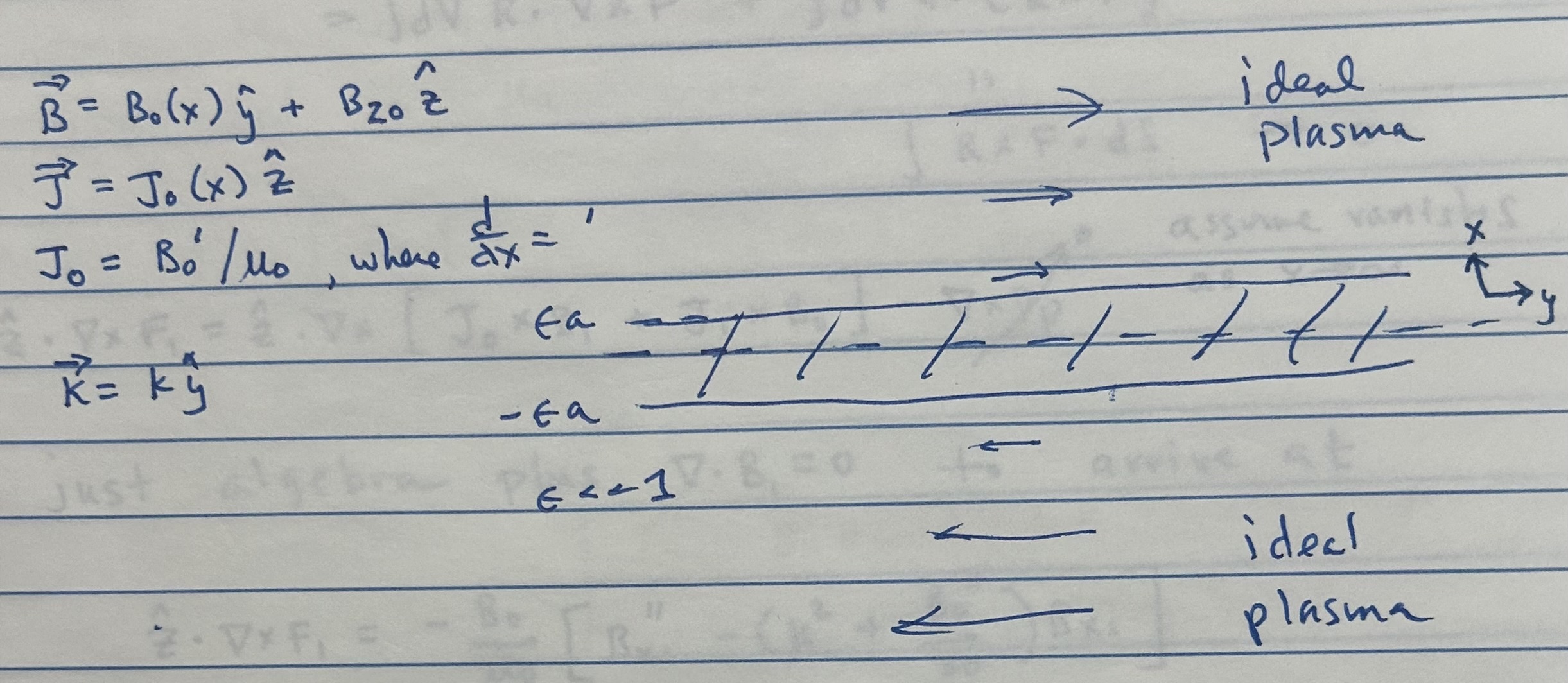
44.5 FKR via Power Flow

We consider a Cartesian slab with equilibrium magnetic field

\bm {B}_0 = B_0(x)\,\hat {\bm y} + B_{z0}\,\hat {\bm z},

and equilibrium current

\bm {J}_0 = J_0(x)\,\hat {\bm z}, \qquad J_0 = \frac {1}{\mu _0}\frac {dB_0}{dx}.

Perturbations are taken of the form

\sim e^{\gamma t + i k y},

with wavevector $\bm {k}=k\hat {\bm y}$.

We assume incompressibility,

\nabla \cdot \bm {v}_1=0,

and adopt a vector–potential representation for the perturbed velocity,

\bm {v}_1=\nabla \times \phi \bm {e}_z

Steps:

1.: Evaluate $P = \int dV \bm {F} \cdot \bm {v}$, where $\bm {F} = \bm {J}\times \bm {B} - \nabla p$. If $P>0\rightarrow $ instability.
2.: Use scale separation for a boundary layer problem to connect "inner" to "outer" solution.
3.: Use MHD eqn’s to relate $\bm {v}_1$ and $\bm {B}_1$ perturbations in inner region
4.: Find growth rate, $\gamma $, for linear solution.

Follow the Energy The work done by the perturbed force is

P=\int dV\,\bm {F}\cdot \bm {v}_1, \qquad \bm {F}=\bm {J}\times \bm {B}-\nabla p .

Instability corresponds to $P>0$.

Using the vector identities

\begin{aligned}P &= \int dV\,\bm {F}\cdot \vect {v} \nonumber \\ &= \int dV\,\bm {F}\cdot (\nabla \times \phi \vect {e}_z) \nonumber \\ &= \int dV\,\phi \vect {e}_z \cdot (\nabla \times \bm {F}) + \oint d\bm {S}\cdot (\phi \vect {e}_z\times \bm {F}).\end{aligned}

Assuming perturbations vanish at infinity, the surface term is zero.

Linearizing the force and using $\nabla \cdot \bm {B}_1=0$,

\vect {e}_z \cdot \nabla \times \bm {F}_1 = \vect {e}_z \cdot \nabla \times (\bm {J}_0\times \bm {B}_1 +\bm {J}_1\times \bm {B}_0 -\nabla p )

straightforward algebra yields

\vect {e}_z \cdot \nabla \times \bm {F}_1 = -\frac {B_0}{\mu _0} \left [ B_{x1}'' - \left (k^2+\frac {B_0''}{B_0}\right )B_{x1} \right ].

The velocity and magnetic perturbations are related through the induction equation,

\partial _t \bm {B}_1 = \nabla \times (\bm {v}_1\times \bm {B}_0) - \frac {\eta }{\mu _0}\nabla ^2\bm {B}_1 .

In the outer ideal region resistivity is negligible, giving

\gamma B_{x1}=ikB_0 v_{x1},

so that

\phi =\frac {v_{x1}}{ik} = \frac {\gamma }{k^2B_0}B_{x1}.

Substituting into the power integral gives

P = \int _{-\infty }^{\infty }dx\, \frac {\gamma }{\mu _0 k^2} B_{x1} \left [ B_{x1}''- \left (k^2+\frac {B_0''}{B_0}\right )B_{x1} \right ].

Outer Ideal Region and $\Delta '$ In the ideal outer region inertia is negligible and $\bm {F}\approx 0$, so the governing equation becomes

B_{x1}''- \left (k^2+\frac {B_0''}{B_0}\right )B_{x1}=0.

This equation is singular at the resonant surface $x=0$, where $B_0=0$ at $x=0$. Hence, the contribution to power is concentrated in the inner region, and thus the energy flow from magnetic field into plasma is all in the inner layer:

P = \int _{-\infty }^{\infty }[...]dx\ \simeq \int _{-\epsilon a}^{\epsilon a }[...]dx

Across this layer:

$B_{x1}$ is continuous,
$dB_{x1}/dx$ is discontinuous due to the sheet current.
In the constant–$\psi $ approximation we take $B_{x1}\approx B_{x1}(0)$ across the inner layer.
expect gradients $\frac {d}{dx}$ to dominate.

\begin{aligned}P & \approx \int _{-\epsilon a}^{\epsilon a } \frac {\gamma }{\mu _0 k^2} B_{x1}(0) \frac {\partial ^2 B_{x1}}{\partial x^2} dx \\ & = \frac {\gamma }{\mu _0 k^2} B_{x1}^2(0) \underbrace {\frac {1}{B_{x1}(0)} \left \{ \left .\frac {dB_{x1}}{dx}\right |_{\epsilon a} - \left . \frac {dB_{x1}}{dx}\right |_{-\epsilon a} \right \}}_{\equiv \Delta '}\end{aligned}

Define the tearing stability parameter

\Delta ' = \frac {1}{B_{x1}(0)} \left [ \left .\frac {dB_{x1}}{dx}\right |_{0^+} - \left .\frac {dB_{x1}}{dx}\right |_{0^-} \right ].

Evaluating the power integral across the thin inner region gives

P= \frac {\gamma B_{x1}^2(0)}{\mu _0 k^2}\Delta '.

Thus

\Delta '>0 \quad \Rightarrow \quad P>0,

which implies instability. First solved by Furth, Kileen and Rosenbluth, hence goes by "FKR" Furth et al. (1963) Importantly, stability is determined entirely by the outer ideal solution; the growth rate depends on the inner region physics.

Solving for the Inner Resistive Layer Inside the inner layer neither inertia nor resistivity can be neglected.

First, lets deal with inertia that we neglected in the linearized momentum equation:

\begin{aligned}\hat {\bm {z}}\cdot \nabla \times \left [ \rho \frac {d\bm {v}}{dt} \right ] & = \hat {\bm {z}}\cdot \nabla \times \left (\rho (\partial _t \bm {v} + \cancel { \bm {v} \cdot \nabla \bm {v}})\right ) \\ \rho \,\partial _t(\nabla \times \bm {v}_1)_z & = \rho \gamma \left (\frac {dv_{y1}}{dx}-ikv_{x1}\right ),\end{aligned}

and incompressibility implies

v_{y1}=-\frac {1}{ik}\frac {dv_{x1}}{dx}.

so that

\begin{aligned}\hat {\bm {z}}\cdot \nabla \times \left [ \rho \frac {d\bm {v}}{dt} \right ] & = \rho \gamma \left (\frac {-1}{ik} \frac {d^2v_{x1}}{dx^2}-ikv_{x1}\right ), \\ & = \frac {i \rho \gamma }{k} \left ( \frac {d^2v_{x1}}{dx^2}-k^2v_{x1}\right ).\end{aligned}

Combining with previous result:

\frac {i \rho \gamma }{k} \left ( \frac {d^2v_{x1}}{dx^2}-k^2v_{x1}\right )= -\frac {B_0}{\mu _0} \left [ B_{x1}'' - \left (k^2+\frac {B_0''}{B_0}\right )B_{x1} \right ].

From the $\hat {\bm {x}}$ component of the magnetic induction equation

\hat {\bm {x}} \cdot \left [ \partial _t \bm {B}_1 = \nabla \times (\bm {v}_1 \times \bm {B}_0) - \frac {\eta }{\mu _0} \nabla ^2 \bm {B}_1\right ]

arrive at

\gamma B_{x1} = i k B_0 v_{x1} + \frac {\eta }{\mu _0} \left ( B_{x1}^{\prime \prime } - k^2 B_{x1}\right )

Combining with the induction equation,

\gamma B_{x1} = ikB_0 v_{x1} + \frac {\eta }{\mu _0}\left (B_{x1}''-k^2B_{x1}\right ).

Using the constant–$\psi $ approximation and eliminating $B_{x1}''$, one finds the inner-layer balance leading to the classical FKR scaling.

\rho \left (v_{x1}''-k^2 v_{x1}\right ) - \frac {k^2 B_0^2}{\gamma \eta }\,v_{x1} = \frac {ik}{\gamma \eta } \left ( \gamma -\frac {\eta }{\mu _0}\frac {B_0''}{B_0} \right ) B_{x1}(0)

Dimensional analysis for sheet width:

Note:

B_0(x)\simeq B_0\frac {x}{a} \qquad \Rightarrow \qquad B_0(\pm \epsilon a)=\pm B_0\epsilon .

Also write

\frac {d^2}{dx^2}\gg k^2 \qquad \text {in the sheet}.

\frac {1}{(\epsilon a)^2} \sim \frac {k^2 \epsilon ^2 B_0^2}{\rho \gamma \eta } \qquad \text {or}\qquad \frac {1}{(\epsilon a)^4} \sim \frac {k^2 B_0^2}{\rho \gamma \eta a^2}.

Isolate growth rate by balancing power driven from ideal region with ohmic dissipation in the sheet.

P_\Omega =\int dV\,\eta J^2 \simeq \epsilon a\,\eta J_{z1}^2(0)

\mu _0 J_{z1} = \frac {\partial B_{y1}}{\partial x} \sim \frac {B_{y1}(\epsilon a)-B_{y1}(-\epsilon a)}{\epsilon a}

From $\nabla \cdot \bm {B}_1=0$,

ik B_{y1}=\frac {dB_{x1}}{dx}.

\mu _0 J_{z1} \simeq \frac { \left .\dfrac {dB_{x1}}{dx}\right |_{\epsilon a} - \left .\dfrac {dB_{x1}}{dx}\right |_{-\epsilon a} } {ik\,\epsilon a} = \frac {B_{x1}(0)}{ik\,\epsilon a}\Delta '.

So that the total power (by this method) is

P_\Omega = \frac {\epsilon a \eta }{\mu _0^2} \frac {B_{x1}^2(0) \Delta '^2}{k^2 \epsilon ^2 a^2}

FKR Growth Rate from Power Balance Equating power input to resistive dissipation yields

\frac {\gamma B_{x1}^2(0)}{\mu _0 k^2}\Delta ' = \frac {\epsilon a \eta }{\mu _0^2} \frac {B_{x1}^2(0) \Delta '^2}{k^2 \epsilon ^2 a^2}

so that the growth rate

\gamma = \frac {\eta }{\mu _0}\frac {\Delta '}{\epsilon a}.

Using the previous result for $(\epsilon a)^4$

\gamma ^4 =(\eta /\mu _0)^4 \Delta '^4 \frac {k^2 B_0^2}{\rho \gamma \eta a^2}

Thus,

\gamma = \left (\frac {k^2 B_0^2}{\mu _0\rho a^2}\right )^{1/5} \left (\frac {\eta }{\mu _0}\right )^{3/5} \Delta '^{4/5}.

Introducing the Alfvén time

\tau _A=\frac {a}{V_A}=\frac {a\sqrt {\mu _0\rho }}{B_0},

the resistive diffusion time

\tau _R=\frac {\mu _0 a^2}{\eta },

and the Lundquist number $S=\tau _R/\tau _A$, the growth rate may be written

\gamma \tau _A = (\Delta 'a)^{4/5}S^{-3/5}(ka)^{2/5}.

Takeaways

What this appendix should leave behind.

The slab sheet pinch is the simplest matched-asymptotic resistive-MHD problem.

The tearing branch is even in $\psi $, forms islands, and is governed by the non-local matching parameter $\Delta '$.

The rippling branch is odd in $\psi $, does not reconnect at leading order, and is driven by current crossing resistivity gradients.

The gravitational branch is also odd in $\psi $, is buoyancy-like, and exhibits the characteristic $\eta ^{1/3}$ resistive-interchange scaling.

The cylindrical tearing and resistive-interchange lectures are best read as geometric refinements of this same basic slab logic.

Bibliography

Harold P. Furth, John Killeen, and Marshall N. Rosenbluth. Finite-resistivity instabilities of a sheet pinch. Physics of Fluids, 6(4):459–484, 1963. doi:10.1063/1.1706761.

K. V. Roberts and J. B. Taylor. Gravitational resistive instability of an incompressible plasma in a sheared magnetic field. Physics of Fluids, 8(2):315–322, 1965. doi:10.1063/1.1761225.

Bruno Coppi, John M. Greene, and John L. Johnson. Resistive instabilities in a diffuse linear pinch. Nuclear Fusion, 6(2):101–117, 1966. doi:10.1088/0029-5515/6/2/003.

Problems

Problem 44.1.: Starting from Eqs. (J.8)–(J.10), derive the reduced slab equations (J.11) and (J.12) in detail.
Problem 44.2.: For the Harris sheet (J.18), solve the outer equation (J.19) and verify Eq. (J.20).
Problem 44.3.: Using the parity assignments (J.21) and (J.22), show directly from Eq. (J.24) why the tearing branch forms islands while the rippling and interchange branches do not.
Problem 44.4.: Recover the dimensional estimates in Eqs. (J.25) and (J.31) by balancing induction, field-line bending, and either outer matching (for tearing) or buoyancy (for the gravitational branch).