Why this lecture matters. A dynamo is not just “a magnetic field in motion.” It is a
conducting flow that amplifies magnetic energy fast enough to outrun resistive diffusion. This
lecture has four jobs:
1.
restate the induction equation as an eigenvalue problem for magnetic growth;
2.
show, with the algebra visible, how stretching competes with diffusion;
3.
derive the axisymmetric flux-function equations and explain Cowling’s theorem; and
4.
introduce the mean-field \(\alpha \)–\(\Omega \) closure that reopens the door once strict axisymmetry is
relaxed.
In the Lectures 6, 7 and 17 the presence of a magnetic field is taken as given for each
astrophysical geometry presenting a "chicken-and-egg" dilemma which is the topic of this
lecture.
Persistent planetary and stellar magnetic fields are the classical evidence that conducting flows can do
more than passively advect flux. Left to itself, the magnetic field would decay on the resistive time \(\tau _\lambda \sim L^2/\lambda \), where \[ \lambda \equiv \frac {\eta }{\muo } = \frac {1}{\muo \sigma } \]
is the magnetic diffusivity associated with the resistive Ohm’s law (1.9). Yet the Earth, the Sun, and many
laboratory flows sustain magnetic structure far longer than that. The central question of dynamo theory is
therefore precise: can the inductive term in (1.13) create magnetic energy faster than diffusion destroys
it?
Historical Perspective
Larmor’s 1919 proposal that solar magnetism might be self-excited by fluid motion
posed the right question before the mathematical tools were ready [Larmor, 1919].
Cowling’s anti-dynamo theorem then supplied an equally important negative result:
strict axisymmetry cannot do the job [Cowling, 1933]. Very quickly, however, it became
clear that anti-dynamo theorems were not the end of the story but a clue about what a
successful flow must actually do.
Vainshtein and Zel’dovich’s stretch–twist–fold picture isolated the topological core
of fast dynamo action: stretch a flux tube to amplify \(B\), twist it so like-signed flux
can be brought together rather than cancelled, and fold it back into the original
volume so the process can repeat [Vainshtein and Zeldovich, 1972, Moffatt, 1989].
Childress and Gilbert later turned that cartoon into a full language for fast dynamos
[Childress and Gilbert, 1995]. In parallel, Bullard and Gellman translated the kinematic
problem into a practical spectral calculation in spherical geometry [Bullard and
Gellman, 1954], Dudley and James showed that smooth flows in a sphere can
realize the same logic without literal folded ropes [Dudley and James, 1989], and
Parker introduced the mean-field \(\alpha \) effect that closes the loop for stars [Parker, 1955].
Liquid-metal experiments then demonstrated that self-excitation is not merely
astrophysical rhetoric, while simultaneously forcing everyone to confront threshold,
saturation, symmetry breaking, and turbulence as dynamo problems in their own
right [Stieglitz and Müller, 2001, Müller et al., 2008, Monchaux et al., 2007, Spence
et al., 2005, Nornberg et al., 2006].
8.1 The kinematic dynamo problem
Induction equation and the eigenvalue viewpoint.
We start from the induction equation derived in the introduction, Eq. (1.13):
The kinematic dynamo approximation treats \(\uvec (\xvec ,t)\) as prescribed and neglects the Lorentz-force back reaction in
(1.8). One then asks whether (8.2) admits growing modes of the form
A positive real part, \(\Re (\gamma )>0\), means magnetic self-excitation. If \(\uvec =0\), the eigenproblem reduces to pure diffusion and
every mode decays.
It is useful to compare the advective time and the resistive time: \[ \tau _u \sim \frac {L}{U}, \qquad \tau _\lambda \sim \frac {L^2}{\lambda }, \qquad \mathrm {Rm}\equiv \frac {\tau _\lambda }{\tau _u} = \frac {UL}{\lambda }. \] Large \(\mathrm {Rm}\) is the regime in which advection
dominates diffusion and the field is approximately frozen to the flow in the sense of (2.13). Equation (2.7)
already showed that the field is stretched by velocity gradients when diffusion is weak. But flux freezing
alone does not guarantee growth. A dynamo needs a velocity field that repeatedly stretches and reorients
the field, not just one that carries it around.
Why stretching matters: the magnetic-energy equation.
The algebra becomes much clearer if we expand the induction term. Using the identity \[ \curl (\uvec \times \B ) = \uvec (\divergence \B ) - \B (\divergence \uvec ) + (\B \cdot \grad )\uvec - (\uvec \cdot \grad )\B , \] and imposing \(\divergence \B =0\), we
obtain
This is the cleanest kinematic statement of the problem. The first term is magnetic-line stretching by the
strain field. The second is Joule dissipation. A dynamo requires the first to beat the second on
average.
Caution
Large \(\mathrm {Rm}\) is necessary, not sufficient. Equation (8.14) says that magnetic energy grows
only if the field samples a velocity gradient with the right geometry. Two-dimensional
stirring, purely axisymmetric motion, or motions with the wrong symmetry can have
very large \(\mathrm {Rm}\) and still fail as dynamos. In the large-\(\mathrm {Rm}\) limit, growth typically proceeds by
stretching the field to small scales until the weak diffusion neglected in (2.8) becomes
important again.
Stretch–twist–fold as the irreducible cartoon.
The most compact way to see why stretching matters is to compare magnetic evolution with the evolution
of a material line element. In ideal incompressible MHD, (8.6) reduces to
Equations (8.15) and (8.16) are the same equation. In that precise sense, ideal MHD says that magnetic
field lines are stretched exactly as material line elements are stretched.
Now take an incompressible flux tube of length \(L\), cross-sectional area \(A\), and magnetic flux \(\Phi = BA\). If the
flow stretches the tube to a new length \(L'=\alpha L\) while approximately conserving volume, then \[ A' L' = A L \qquad \Rightarrow \qquad A'=\frac {A}{\alpha }. \] Flux
freezing says \(\Phi '=\Phi \), so \[ B' A' = B A \qquad \Rightarrow \qquad B' = \alpha B . \] This is the first step of the Zel’dovich cartoon: stretching alone amplifiesmagnetic field strength. But stretching by itself just produces one longer, thinner tube. To make
a dynamo one must bring amplified flux back into the original domain without destructive
cancellation. That is the role of twist and fold. Twist reorients the tube so that the folded return
strand carries flux in the same direction, and fold reinjects the amplified tube into the original
volume where the process can repeat. Diffusion is still needed, but only in the thin folded
layers where neighboring strands reconnect and the topology can reset. The stretch–twist–fold
picture is therefore not a literal engineering blueprint. It is the minimal kinematic logic of a fast
dynamo.
A smooth realization of stretch–twist–fold: the Dudley–James flow.
Bullard and Gellman introduced the toroidal–poloidal decomposition that makes spherical kinematic
calculations practical [Bullard and Gellman, 1954]. Any solenoidal field can be written as
with analogous expressions for \(\B \). Expanding the scalars \(T\) and \(S\) in spherical harmonics turns (8.4) into a
matrix eigenvalue problem for the mode amplitudes.
Dudley and James identified especially simple flows in a sphere that excite magnetic modes at
comparatively low \(\mathrm {Rm}\) [Dudley and James, 1989, O’Connell et al., 2001]. Their \(T2S2\) flow is built from \(\ell =2\) toroidal
and poloidal pieces,
where \(\epsilon \) controls the relative strength of the poloidal circulation. For the axisymmetric \(\ell =2\) member of this
family, the velocity components are
These flows are useful because one can see, almost by inspection, the ingredients in (8.14): circulation
stretches the field, toroidal motion twists it, and the combined three-dimensional geometry allows folding
and reorientation instead of mere diffusion. Read in stretch–twist–fold language, the poloidal circulation
supplies the repeated stretch-and-return of flux tubes while the toroidal component \(u_\phi \) supplies the twist
that keeps the returned flux aligned rather than cancelled. Dudley and James are important
because they show that the Zel’dovich cartoon is not confined to discrete maps or knotted
ropes. A smooth, divergence-free flow in an ordinary sphere can realize the same topology
continuously.
Experimental perspective.
Kinematic calculations mattered enormously for experiment because liquid-sodium facilities cannot reach
arbitrarily large \(\mathrm {Rm}\). The flow has to be engineered to sit near threshold as efficiently as possible,
but there are very different ways to do that. Karlsruhe deliberately realized a Roberts-type
two-scale dynamo with helical channels, so the experiment was almost a direct embodiment
of a mean-field calculation [Stieglitz and Müller, 2001, Müller et al., 2008]. The Madison
Dynamo Experiment pursued a different philosophy: approximate a smooth spherical two-vortex
flow strongly enough that the predicted magnetic eigenmodes become experimentally relevant
[Spence et al., 2005, Nornberg et al., 2006, Lathrop and Forest, 2011]. From that point of
view, Madison sits much closer to the Dudley–James program than to the helical-pipe logic of
Karlsruhe.
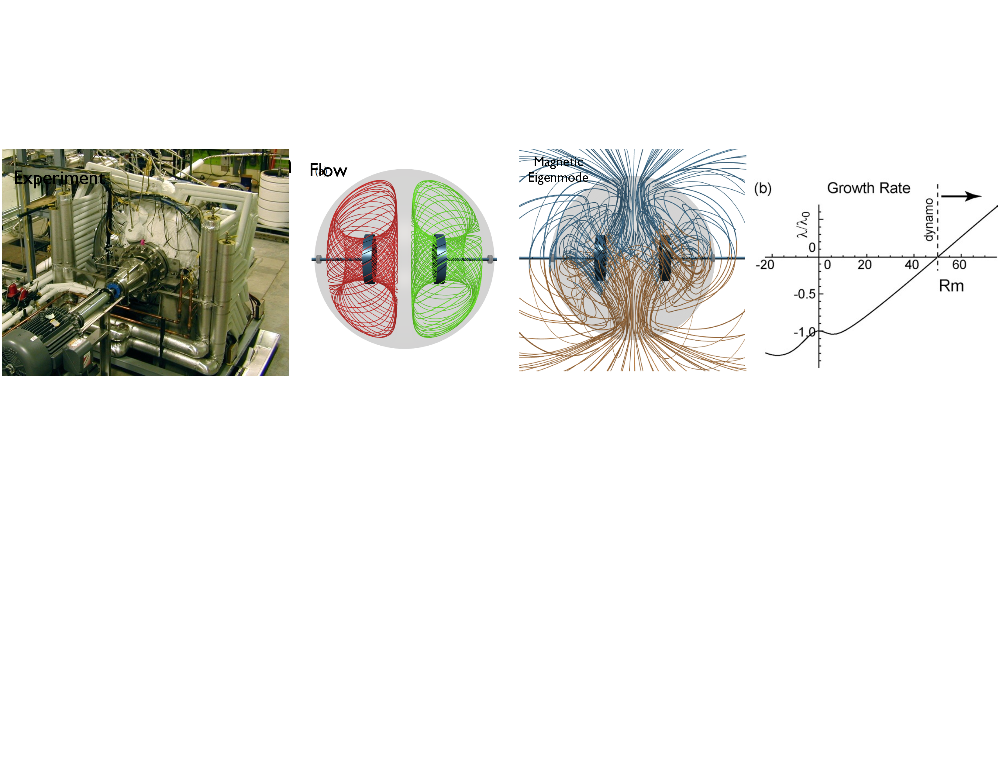
Figure 8.1: The Madison Dynamo Experiment, a \(1~\mathrm {m}\) spherical liquid-sodium device driven by two
counter-rotating propellers. A local field-line movie appears just below this figure. The measured system lived
close to the kinematic threshold, so intermittent excitation and turbulence-induced magnetic fields
became central parts of the story [Spence et al., 2005, Nornberg et al., 2006].
Field-Line Movie
Watch for the three-dimensional stretching and return of field structures that make the Madison flow a smooth laboratory analogue of stretch–twist–fold dynamics.
Movie clip associated with the Madison Dynamo Experiment discussion in this lecture.
The Dudley–James calculation and the Madison device therefore fit together naturally. The calculation
says that a smooth spherical flow with the right mixture of meridional circulation and swirl can be a
dynamo at achievable threshold. The experiment then asks whether a turbulent laboratory flow can stay
close enough to that kinematic target for the corresponding magnetic eigenmode to emerge.
In that sense Madison is not a separate story from stretch–twist–fold. It is an attempt to
realize a smooth three-dimensional stretch–twist–fold surrogate in sodium rather than on a
blackboard.
VKS adds yet another twist. It achieved self-excitation in a violently turbulent von Kármán flow
[Monchaux et al., 2007], but later analysis showed that the observed axisymmetric mode and the dynamo
threshold depended strongly on the magnetic permeability of the soft-iron impellers [Giesecke
et al., 2010]. That is precisely why the experiment became interesting: not because one more kinematic
threshold had been crossed, but because turbulence, symmetry breaking, magnetic boundary conditions,
and nonlinear saturation all became inseparable.
Opinion
Karlsruhe and VKS were genuine milestones, and it would be silly to diminish the
experimental ingenuity required to build them. But they were also highly constrained
realizations of already-favored kinematic ideas. Karlsruhe hard-wired helicity through
helical channels; VKS used impeller geometry and ferromagnetic material that strongly
selected the observed mode. In that limited sense, once the flow topology and magnetic
boundary conditions were engineered correctly, Maxwell’s equations had much less
freedom than the word “dynamo” sometimes suggests.
From this point of view, the deepest discoveries were not merely that self-excitation could
occur, but how the system saturated, how turbulence modified the mean electromotiveforce, and which magnetic symmetries survived the nonlinear state. Madison was
especially valuable on that front because it lived close enough to threshold that
intermittency, fluctuation-driven induction, and turbulent transport became part of the
physics rather than just noise around a predetermined outcome.
8.2 Axisymmetry, flux functions, and Cowling’s theorem
The Stokes function in axisymmetry.
Many geophysical and astrophysical systems are approximately axisymmetric, so it is natural to ask
whether axisymmetry by itself can maintain a magnetic field. In cylindrical coordinates \((r,\phi ,z)\) with \(\pp {}{\phi }=0\), write
This is the same operator that later appears in equilibrium theory. The toroidal current sources poloidal
field; conversely, poloidal current sources toroidal field.
Derivation of the axisymmetric induction equations.
The reason \(\psi \) is so useful is that the toroidal component of Ohm’s law immediately produces a scalar
evolution equation. Start from (1.9), \[ \E + \uvec \times \B = \eta \J , \] and take the \(\phi \) component. Because \(\vect {A} = \psi \grad \phi = (\psi /r)\vect {e}_\phi \), axisymmetry gives
The first curl gives poloidal advection of \(B\), while the second is
Omega-Effect Movie
Watch for how differential rotation shears poloidal structure into toroidal field, building the strong azimuthal component that drives the first half of the alpha-omega loop.
Movie clip paired with the toroidal-field induction and omega-effect discussion in this lecture.
Equation (8.40) says that differential rotation can convert poloidal field into toroidal field. Equation (8.38)
says the reverse process is absent in strict axisymmetry.
Cowling’s theorem.
Cowling’s theorem may now be stated in its physically useful form:
Cowling’s theorem. No purely axisymmetric flow can maintain a purely axisymmetric
magnetic field against resistive decay.
The algebraic heart of the theorem is already visible in (8.38). The equation for \(\psi \) is homogeneous.
Axisymmetric motion can rearrange \(\psi \), and resistivity can dissipate it, but there is no term proportional to \(B\),
\(\Omega \), or any other axisymmetric quantity that creates new poloidal flux. Once \(\psi \) decays, the \(\Omega \)-effect source \(r\B _p\cdot \grad \Omega \) in
(8.40) disappears with it, so the toroidal field also decays.
It is still worth seeing the dissipative sign directly. Multiply (8.38) by \(\psi /r^2\) and integrate over volume:
With homogeneous boundary data or sufficiently rapid decay at infinity, the surface terms vanish, and the
resistive part is strictly non-positive. A mathematically complete proof must handle the transport term
with the correct cylindrical weighting, but the physical conclusion is already fixed by (8.38): in strict
axisymmetry there is diffusion of \(\psi \) and no source for \(\psi \). That is why an axisymmetric \(\Omega \) effect, by itself, never
closes the loop.
8.3 Mean-field closure and the alpha-Omega picture
Averaging and the turbulent electromotive force.
The way out of Cowling’s theorem is not to deny it, but to relax strict axisymmetry. Write \[ \uvec = \overline {\uvec } + \widetilde {\uvec }, \qquad \B = \overline {\B } + \widetilde {\B }, \] where the
overbar denotes an average over fluctuations and \(\langle \widetilde {\uvec } \rangle = \langle \widetilde {\B }\rangle = 0\). Averaging (8.2) gives
The new object \[ \mathcal {E} \equiv \langle \widetilde {\uvec }\times \widetilde {\B }\rangle \] is the mean turbulent electromotive force. Under isotropic first-order smoothing, one
writes
The coefficient \(\alpha \) is nonzero only when the fluctuations break mirror symmetry, usually through rotation
plus stratification or helical forcing.
Alpha-Effect Movie
Watch for how helical motion converts toroidal structure back into poloidal flux, closing the regeneration loop sketched in the alpha-omega cartoon.
Movie clip paired with the alpha-effect and alpha-omega dynamo discussion in this lecture.
The coefficient \(\beta \) acts like an enhanced magnetic
diffusivity. Parker’s great step was to recognize that rotating convection naturally supplies just such a
helical electromotive force [Parker, 1955]. In liquid metal, the same kind of turbulent EMF has even been
measured directly [Rahbarnia et al., 2012].
The axisymmetric \(\alpha \)–\(\Omega \) equations.
Absorb \(\beta \) into an effective diffusivity \(\lambda _T = \lambda + \beta \), and keep only the dominant source terms. Then the axisymmetric
mean-field equations become
These two equations capture the canonical loop: \[ \text {poloidal field} \;\xrightarrow {\;\Omega \;\text {effect}\;} \text {toroidal field} \;\xrightarrow {\;\alpha \;\text {effect}\;} \text {poloidal field}. \] The factor of \(r\) in (8.48) is not decoration. It comes from
the definition \(\vect {A} = \psi \grad \phi = (\psi /r)\vect {e}_\phi \), so the toroidal EMF contributes to \(\pp {\psi }{t}\) through \(r E_\phi \).
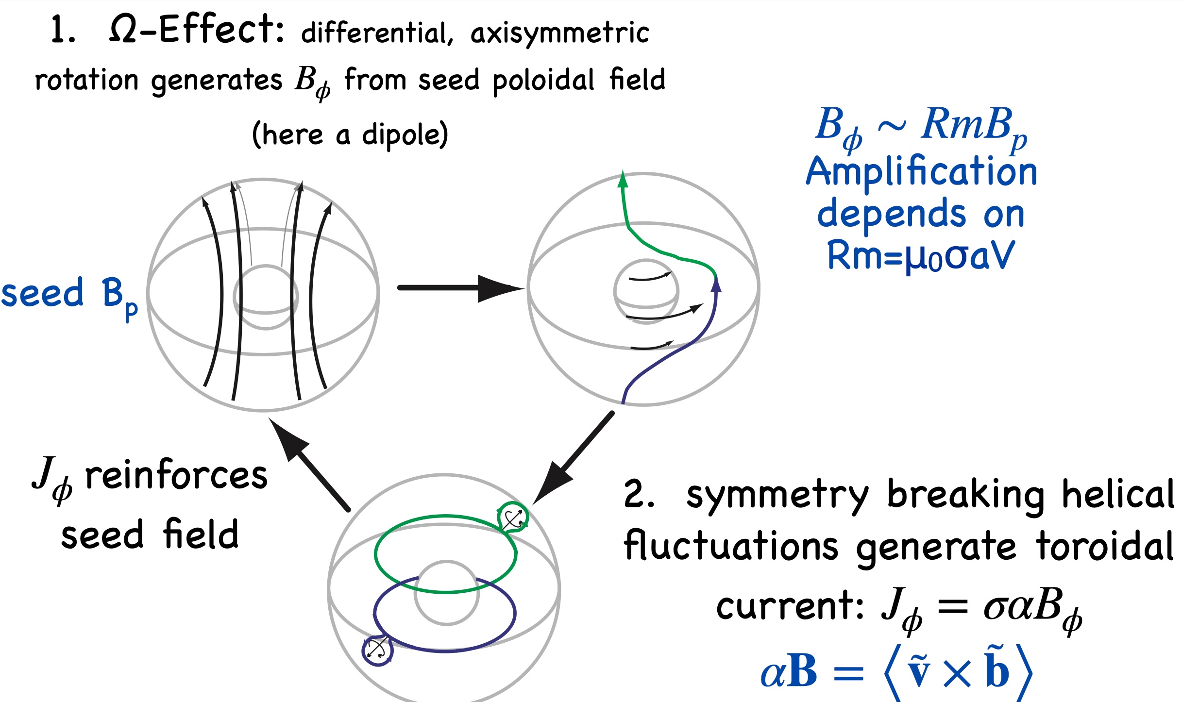
Figure 8.2: The standard \(\alpha \)–\(\Omega \) cartoon: differential rotation winds poloidal field into toroidal field,
while helical fluctuations regenerate poloidal flux from toroidal field.
A local \(\alpha \)–\(\Omega \) estimate.
A simple local model makes the competition between induction and diffusion almost embarrassingly
transparent. Let \(A(x,t)\) be a local toroidal vector potential so that the mean poloidal field is obtained from \(A\), and
let \(B(x,t)\) be the mean toroidal field. Suppose the large-scale shear is \(G \equiv \dd {U_y}{x}\), and retain only one spatial coordinate.
Then
Now look for normal modes, \[ A,\,B \propto e^{\gamma t + i k x}. \] Equations (8.50) and (8.51) become
\[(\gamma + \lambda _T k^2)A = \alpha B, \qquad (\gamma + \lambda _T k^2)B = i k G A.\]
Eliminate either \(A\) or \(B\):
\[(\gamma + \lambda _T k^2)^2 = i\alpha G k . \tag{8.53}\]
Thus the growth rate is determined by the square root of \(i\alpha G k\). The important point is immediate even before
taking the square root explicitly:
diffusion appears only through the stabilizing shift \(+\lambda _T k^2\),
dynamo action disappears if either \(\alpha =0\) or \(G=0\), and
the complex right-hand side implies oscillatory propagation as well as growth or decay.
This is the local seed of Parker’s dynamo-wave picture.
What to remember physically.
The dynamo problem is not solved by one mechanism alone. Stretching without topology change piles field
into ever smaller scales until diffusion wins. Diffusion without stretching simply erases the field. The
classical success of mean-field theory was to show how symmetry-breaking fluctuations can systematically
regenerate the large-scale part of the field while shear builds strong toroidal components. Whether that
closure is quantitatively adequate is a separate, harder question, but the architecture of the problem is
already visible in (8.48) and (8.49).
Takeaways
1.
The kinematic dynamo problem is the eigenvalue problem (8.4): can induction
overcome diffusion for a prescribed flow?
2.
The magnetic-energy balance (8.14) and the line-element equation (8.16) show
exactly what growth requires: stretching must beat Joule dissipation, while twisting
and folding prevent the amplified flux from cancelling itself.
3.
The stretch–twist–fold cartoon is the minimal topological logic of a fast dynamo;
Dudley–James flows show how that same logic appears in smooth spherical advection,
and Madison was built to chase that smooth version experimentally.
4.
In axisymmetry, the poloidal flux equation (8.38) contains advection and diffusion
but no source. That is the operational content of Cowling’s theorem.
5.
The mean-field \(\alpha \)–\(\Omega \) model reintroduces a source for poloidal flux through the turbulent
EMF \(\mathcal {E}=\langle \widetilde {\uvec }\times \widetilde {\B }\rangle \), leading to (8.48)–(8.49).
Bibliography
J. Larmor. Possible rotational origin of magnetic fields of sun and earth. Elec. Rev, 85:412, 1919.
T. G. Cowling. The magnetic field of sunspots. Monthly Notices of the Royal Astronomical Society, 94(1):39–48, 1933. doi:10.1093/mnras/94.1.39.
S. I. Vainshtein and Ya. B. Zeldovich. Origin of magnetic fields in astrophysics (turbulent "dynamo" mechanisms). Soviet Physics Uspekhi, 15(2):159–172, 1972. doi:10.1070/PU1972v015n02ABEH004960.
H. K. Moffatt. Stretch, twist and fold. Nature, 341(6240):285–286, 1989. doi:10.1038/341285a0.
Stephen Childress and Andrew D. Gilbert. Stretch, Twist, Fold: The Fast Dynamo, volume 37 of Lecture Notes in Physics Monographs. Springer, Berlin, Heidelberg, 1995. doi:10.1007/978-3-540-44778-8.
Edward Crisp Bullard and H. Gellman. Homogeneous dynamos and terrestrial magnetism. Philosophical Transactions of the Royal Society of London. Series A, Mathematical and Physical Sciences, 247(928):213–278, 1954. doi:10.1098/rsta.1954.0018.
M. L. Dudley and Reginald William James. Time-dependent kinematic dynamos with stationary flows. Proceedings of the Royal Society of London. A. Mathematical and Physical Sciences, 425(1869):407–429, 1989. doi:10.1098/rspa.1989.0112.
E. N. Parker. Hydromagnetic dynamo models. Astrophysical Journal, 122:293–314, 1955. doi:10.1086/146087.
Robert Stieglitz and Ulrich Müller. Experimental demonstration of a homogeneous two-scale dynamo. Physics of Fluids, 13(3):561–564, 2001. doi:10.1063/1.1331315.
Ulrich Müller, Robert Stieglitz, Fritz H. Busse, and Andreas Tilgner. The karlsruhe two-scale dynamo experiment. Comptes Rendus Physique, 9(7):729–740, 2008. doi:10.1016/j.crhy.2008.07.005.
Romain Monchaux, Michael Berhanu, Mickael Bourgoin, et al. Generation of a magnetic field by dynamo action in a turbulent flow of liquid sodium. Physical Review Letters, 98:044502, 2007. doi:10.1103/PhysRevLett.98.044502.
E J Spence, M D Nornberg, C M Jacobson, R D Kendrick, and C B Forest. Observation of a turbulence-induced large scale magnetic field. Physical Review Letters, 96(5):055002, 2005. doi:10.1103/physrevlett.96.055002.
M D Nornberg, E J Spence, R D Kendrick, C M Jacobson, and C B Forest. Intermittent magnetic field excitation by a turbulent flow of liquid sodium. Physical Review Letters, 97(4):044503, 2006. doi:10.1103/physrevlett.97.044503.
R. O'Connell, Roch Kendrick, Mark Nornberg, Erik Spence, Adam Bayliss, and C. B. Forest. On the possibility of an homogeneous MHD dynamo in the laboratory. In P. Chossat, D. Ambruster, and I. Oprea, editors, Dynamo and Dynamics, a Mathematical Challenge, volume 26 of NATO Science Series II: Mathematics, Physics and Chemistry, pages 59–66. Springer, Dordrecht, 2001. doi:10.1007/978-94-010-0788-7_7.
Daniel P. Lathrop and Cary B. Forest. Magnetic dynamos in the lab. Physics Today, 64(7):40–45, 2011. doi:10.1063/pt.3.1166.
André Giesecke, Frank Stefani, and Günter Gerbeth. Role of soft-iron impellers on the mode selection in the von kármán-sodium dynamo experiment. Physical Review Letters, 104:044503, 2010. doi:10.1103/PhysRevLett.104.044503.
Kian Rahbarnia, Benjamin P Brown, Mike M Clark, Elliot J Kaplan, Mark D Nornberg, Alex M Rasmus, Nicholas Zane Taylor, Cary B Forest, Frank Jenko, Angelo Limone, Jean-François Pinton, Nicolas Plihon, and Gautier Verhille. Direct observation of the turbulent EMF and transport of magnetic field in a liquid sodium experiment. The Astrophysical Journal, 759(2):80, 2012. doi:10.1088/0004-637x/759/2/80.
Problems
Problem 8.1. Kinematic growth, Cowling’s theorem, and mean-field closure
(a)
Starting from the induction equation (8.2), derive the convective form (8.5). Then assume \(\divergence \uvec =0\), dot
the result with \(\B /\muo \), and derive the integrated magnetic-energy balance (8.14). Which term can
make the magnetic energy grow?
(b)
In axisymmetry, define the poloidal flux function by \[ \B _p = \curl (\psi \grad \phi ). \] Derive (8.28) and show explicitly that \(\B _p\cdot \grad \psi =0\).
Then use Ampère’s law to derive (8.32).
(c)
Use the toroidal component of Ohm’s law to derive the axisymmetric flux equation (8.38).
Explain in words why this equation already contains the essence of Cowling’s theorem, even
before one proves a formal decay theorem.
(d)
Consider the local \(\alpha \)–\(\Omega \) system (8.50)–(8.51). Insert \[ A,\,B \propto e^{\gamma t + i k x} \] and derive the dispersion relation (8.53).
Under what conditions does the mode grow rather than decay?
(e)
Let \(\delta \xvec \) be a material line element connecting neighboring fluid parcels. Starting from \[ \frac {D \xvec }{Dt}=\uvec (\xvec ,t), \] derive
(8.16). Then compare it with the ideal incompressible induction equation (8.15) and explain, in
your own words, why stretch amplifies the field, why twist is needed to avoid cancellation after
folding, and which pieces of the Dudley–James flow play those roles most naturally.