Lecture 10
The Grad–Shafranov Equation and the Solov’ev Solution
Overview
Axisymmetry turns vector force balance into one scalar elliptic equation.
-
1.
- In the isotropic limit of the previous lecture, pressure becomes a flux function: \(p=p(\psi )\).
-
2.
- Axisymmetry allows the magnetic field to be written in terms of one poloidal flux
function \(\psi (R,Z)\) and one toroidal-field function \(F(\psi )\).
-
3.
- The Grad–Shafranov equation then determines the shape of flux surfaces once the
boundary and the free functions \(p(\psi )\) and \(F(\psi )\) are specified.
The previous lecture kept the pressure tensor general and asked what static balance looks like in a
gyrotropic plasma. This lecture now makes two deliberate simplifications. First, we return to scalar
pressure, so that Eq. (9.11) collapses to Eq. (9.19). Second, we impose axisymmetry. Those two choices
are enough to reduce the vector equation \(\J \times \B =\grad p\) to a single second-order partial differential equation for the
poloidal flux function.
Historical Perspective
The Grad–Shafranov equation was one of the decisive conceptual advances of
magnetic-confinement theory. Shafranov formulated the toroidal equilibrium problem in
a way that made the role of current, pressure, and geometry transparent, while Grad
emphasized the central importance of flux coordinates and the mathematical structure
of the axisymmetric confinement problem Shafranov [1958, 1960, 1966], Grad [1967].
Nearly every modern tokamak equilibrium code still lives inside this framework, even
when dressed up with sophisticated numerics and diagnostic constraints.
Caution
This lecture is intentionally isotropic. The fully anisotropic equilibrium problem
from the previous lecture does not reduce to the same one-function equation. Once the
pressure depends separately on \(p_\perp \) and \(p_\parallel \), the structure of the equilibrium changes. Here we
are solving the classical isotropic axisymmetric problem.
10.1 Axisymmetry and the flux function
Represent the field so that divergence-free structure is automatic.
In cylindrical coordinates \((R,\phi ,Z)\), axisymmetry means \[ \pp {}{\phi }=0. \] A convenient representation of the magnetic field is
\[\boxed { \B = \grad \psi \times \grad \phi + F(R,Z)\,\grad \phi . } \tag{10.1}\]
Because \(\grad \phi =\ephi /R\), this may also be written as \[\B = -\frac {1}{R}\pp {\psi }{Z}\eR + \frac {F}{R}\ephi + \frac {1}{R}\pp {\psi }{R}\eZ . \tag{10.2}\]
The first and third terms are the poloidal field; the middle term is the toroidal field.
Why psi deserves to be called a flux function.
Contours of constant \(\psi \) in the \((R,Z)\) plane are magnetic surfaces. Indeed,
\[\B \cdot \grad \psi = \left (\grad \psi \times \grad \phi \right )\cdot \grad \psi + F\,\grad \phi \cdot \grad \psi =0,\]
so field lines lie on \(\psi ={\rm constant}\). Up to the conventional factor of \(2\pi \), \(\psi \) is the poloidal magnetic flux enclosed by that
surface.
Compute the current density from Ampère’s law.
Using Eq. (1.11),
\[\muo \J =\curl \B .\]
Insert Eq. (10.2). The toroidal component is \[\begin {aligned} \muo J_\phi &= \pp {B_R}{Z}-\pp {B_Z}{R} \\ &= -\pp {}{Z}\left (\frac {1}{R}\pp {\psi }{Z}\right ) - \pp {}{R}\left (\frac {1}{R}\pp {\psi }{R}\right ) \\ &= -\frac {1}{R} \left [ R\pp {}{R}\left (\frac {1}{R}\pp {\psi }{R}\right ) + \pp {^2\psi }{Z^2} \right ]. \end {aligned}\]
This motivates the definition \[\boxed { \Delta ^\star \psi \equiv R\pp {}{R}\left (\frac {1}{R}\pp {\psi }{R}\right ) + \pp {^2\psi }{Z^2} = \pp {^2\psi }{R^2}-\frac {1}{R}\pp {\psi }{R}+\pp {^2\psi }{Z^2}. } \tag{10.6}\]
Hence \[\boxed { J_\phi =-\frac {1}{\muo R}\Delta ^\star \psi . } \tag{10.7}\]
The poloidal current components come from the remaining curls: \[J_R=-\frac {1}{\muo R}\pp {F}{Z}, \qquad J_Z=\frac {1}{\muo R}\pp {F}{R}, \tag{10.8}\]
so in vector form \[\muo \J = \frac {1}{R}\grad F\times \ephi - \frac {1}{R}\Delta ^\star \psi \,\ephi . \tag{10.9}\]
10.2 Derive the Grad–Shafranov equation step by step
Start from isotropic static force balance.
For scalar pressure, Eq. (1.8) reduces in static equilibrium to
\[\J \times \B =\grad p. \tag{10.10}\]
This is the isotropic specialization of the more general equilibrium equation developed in the previous
lecture.
First show that pressure is a flux function.
Dot Eq. (10.10) with \(\B \):
\[\B \cdot \grad p = \B \cdot (\J \times \B )=0.\]
Thus pressure is constant along field lines. Since field lines lie on \(\psi ={\rm constant}\), one concludes \[\boxed {p=p(\psi ).} \tag{10.12}\]
This is exactly the isotropic statement anticipated in Eq. (9.19).
Next show that the toroidal-field function is also a flux function.
The right-hand side of Eq. (10.10) has no toroidal component, so the toroidal component of \(\J \times \B \) must vanish:
\[(\J \times \B )_\phi =0.\]
Using Eqs. (10.2) and (10.8), \[\begin {aligned} (\J \times \B )_\phi &= J_Z B_R - J_R B_Z \\ &= \frac {1}{\muo R}\pp {F}{R} \left (-\frac {1}{R}\pp {\psi }{Z}\right ) - \left (-\frac {1}{\muo R}\pp {F}{Z}\right ) \frac {1}{R}\pp {\psi }{R} \\ &= \frac {1}{\muo R^2} \left [ \pp {F}{Z}\pp {\psi }{R} - \pp {F}{R}\pp {\psi }{Z} \right ]. \end {aligned}\]
Therefore \[\pp {F}{Z}\pp {\psi }{R}-\pp {F}{R}\pp {\psi }{Z}=0.\]
The gradients \(\grad F\) and \(\grad \psi \) are therefore parallel, so \[\boxed {F=F(\psi ).} \tag{10.16}\]
Once this is true, \[\grad F = F'(\psi )\grad \psi . \tag{10.17}\]
Now write the current in flux-surface form.
Equation (10.9) becomes
\[\J = \frac {F'(\psi )}{\muo R}\grad \psi \times \ephi - \frac {1}{\muo R}\Delta ^\star \psi \,\ephi . \tag{10.18}\]
It is useful to separate this into poloidal and toroidal pieces, \[\J _p= \frac {F'(\psi )}{\muo R}\grad \psi \times \ephi , \qquad \J _\phi =-\frac {1}{\muo R}\Delta ^\star \psi \,\ephi . \tag{10.19}\]
Likewise, \[\B _p= \frac {1}{R}\grad \psi \times \ephi , \qquad \B _\phi = \frac {F(\psi )}{R}\ephi . \tag{10.20}\]
Compute the poloidal-current/toroidal-field term.
Using Eqs. (10.19) and (10.20),
\[\begin {aligned} \J _p\times \B _\phi &= \left [ \frac {F'}{\muo R}\grad \psi \times \ephi \right ] \times \left [ \frac {F}{R}\ephi \right ] \\ &= \frac {FF'}{\muo R^2} \left [(\grad \psi \times \ephi )\times \ephi \right ]. \end {aligned}\]
Because \(\grad \psi \cdot \ephi =0\), the vector identity \[ (\vect {a}\times \vect {b})\times \vect {b} = -\vect {a} \qquad (\vect {a}\cdot \vect {b}=0,\; \vect {b}\cdot \vect {b}=1) \] gives \[\J _p\times \B _\phi = -\frac {FF'(\psi )}{\muo R^2}\grad \psi . \tag{10.22}\]
Compute the toroidal-current/poloidal-field term.
Again from Eqs. (10.19) and (10.20),
\[\begin {aligned} \J _\phi \times \B _p &= \left [ -\frac {1}{\muo R}\Delta ^\star \psi \,\ephi \right ] \times \left [ \frac {1}{R}\grad \psi \times \ephi \right ] \\ &= -\frac {\Delta ^\star \psi }{\muo R^2} \left [\ephi \times (\grad \psi \times \ephi )\right ]. \end {aligned}\]
Now use \[ \vect {b}\times (\vect {a}\times \vect {b}) = \vect {a} \qquad (\vect {a}\cdot \vect {b}=0,\;\vect {b}\cdot \vect {b}=1), \] so \[\J _\phi \times \B _p = -\frac {\Delta ^\star \psi }{\muo R^2}\grad \psi . \tag{10.24}\]
\[\mu _0 \J _\phi = -\frac {\Delta ^\star \psi }{ R}.\]
Add the two pieces and compare with the pressure gradient.
Since \(\J \times \B =\J _p\times \B _\phi + \J _\phi \times \B _p\), Eqs. (10.22) and (10.24) give
\[\J \times \B = -\frac {1}{\muo R^2} \left [ \Delta ^\star \psi + F(\psi )F'(\psi ) \right ]\grad \psi . \tag{10.26}\]
But Eq. (10.12) implies \[\grad p = p'(\psi )\grad \psi . \tag{10.27}\]
Equating Eqs. (10.26) and (10.27) yields the Grad–Shafranov equation, \[\boxed { \Delta ^\star \psi = -\muo R^2\,p'(\psi ) - F(\psi )F'(\psi ). } \tag{10.28}\]
This is the canonical axisymmetric equilibrium equation.
Read off the toroidal current density.
Combining Eq. (10.28) with Eq. (10.7) gives
\[\boxed { J_\phi = R\,p'(\psi ) + \frac {F(\psi )F'(\psi )}{\muo R}. } \tag{10.29}\]
This is often a more intuitive way to think about the equation: choosing \(p(\psi )\) and \(F(\psi )\) specifies how toroidal
current is distributed in order to satisfy force balance.
10.3 Boundary data, free functions, and what it means to solve the equation
Why the problem is elliptic.
The operator \(\Delta ^\star \) from Eq. (10.6) has the same second-derivative structure as a two-dimensional Laplacian,
modified by the cylindrical geometry. Away from \(R=0\) it is elliptic, which is why the entire plasma column
responds globally when one changes the source or the boundary.
Fixed-boundary equilibria.
In the simplest case one prescribes the plasma domain \(\Omega \) and imposes
\[\psi = \psi _b \qquad \text {on } \partial \Omega . \tag{10.30}\]
The magnetic axis is then determined as an interior point where \[\grad \psi = 0. \tag{10.31}\]
This is the standard mathematical setting for analytic examples and many textbook calculations.
Free-boundary equilibria.
In experiments the plasma boundary is often not known in advance. Instead one writes
\[\psi = \psi _{\rm plasma}+\psi _{\rm coils}, \tag{10.32}\]
and solves simultaneously for the plasma current and the last closed flux surface. This is where
separatrices, X-points, and divertor geometries enter.
The free functions are physical input.
Equation (10.28) does not determine \(p(\psi )\) or \(F(\psi )\); they must be supplied from modeling assumptions, transport
calculations, or experimental constraints. A common parameterization is
\[p'(\psi ) = -\sum _{k=0}^{N} a_k\psi ^k, \qquad F(\psi )F'(\psi ) = -\sum _{k=0}^{M} b_k\psi ^k. \tag{10.33}\]
Different choices generate different equilibrium families.
10.4 Solovév equilibria and analytic shaping
Choose constant source terms.
A particularly useful analytic family follows from the simple choice
\[p'(\psi )=-\frac {C_p}{\muo }, \qquad F(\psi )F'(\psi )=-C_F, \tag{10.34}\]
where \(C_p\) and \(C_F\) are constants. Then Eq. (10.28) becomes \[\Delta ^\star \psi = C_p R^2 + C_F. \tag{10.35}\]
Find a particular solution by trial.
Try
\[\psi _p = aR^4 + bZ^2.\]
Using Eq. (10.6), \[\Delta ^\star (R^4)=8R^2, \qquad \Delta ^\star (Z^2)=2. \tag{10.37}\]
Therefore \[\Delta ^\star \psi _p = 8aR^2+2b.\]
Matching Eq. (10.35) gives \[a=\frac {C_p}{8}, \qquad b=\frac {C_F}{2}.\]
So one particular solution is \[\psi _p = \frac {C_p}{8}R^4 + \frac {C_F}{2}Z^2. \tag{10.40}\]
Add homogeneous solutions to shape the boundary.
The homogeneous equation \(\Delta ^\star \psi _h=0\) admits a polynomial family such as
\[\psi _h = c_0 + c_1 R^2 + c_2\left (R^4-4R^2Z^2\right ). \tag{10.41}\]
Hence a simple Solovév family is \[\boxed { \psi (R,Z) = \frac {C_p}{8}R^4 + \frac {C_F}{2}Z^2 + c_0 + c_1 R^2 + c_2\left (R^4-4R^2Z^2\right ). } \tag{10.42}\]
These constants can be traded for more geometric quantities such as axis position, size, and
elongation.
Special case: only externally imposed toroidal field.
If \(F'(\psi )=0\), then \(C_F=0\) and the toroidal-field function is constant and equal to the applied field. Equation (10.28)
reduces to
\[\Delta ^\star \psi = -\muo R^2 p'(\psi ). \tag{10.43}\]
If \(p'\) is also constant, the particular solution collapses to the \(R^4\) piece alone and all shaping comes from the
homogeneous additions. This is often the cleanest classroom example because one can see directly how
pressure drives poloidal flux.
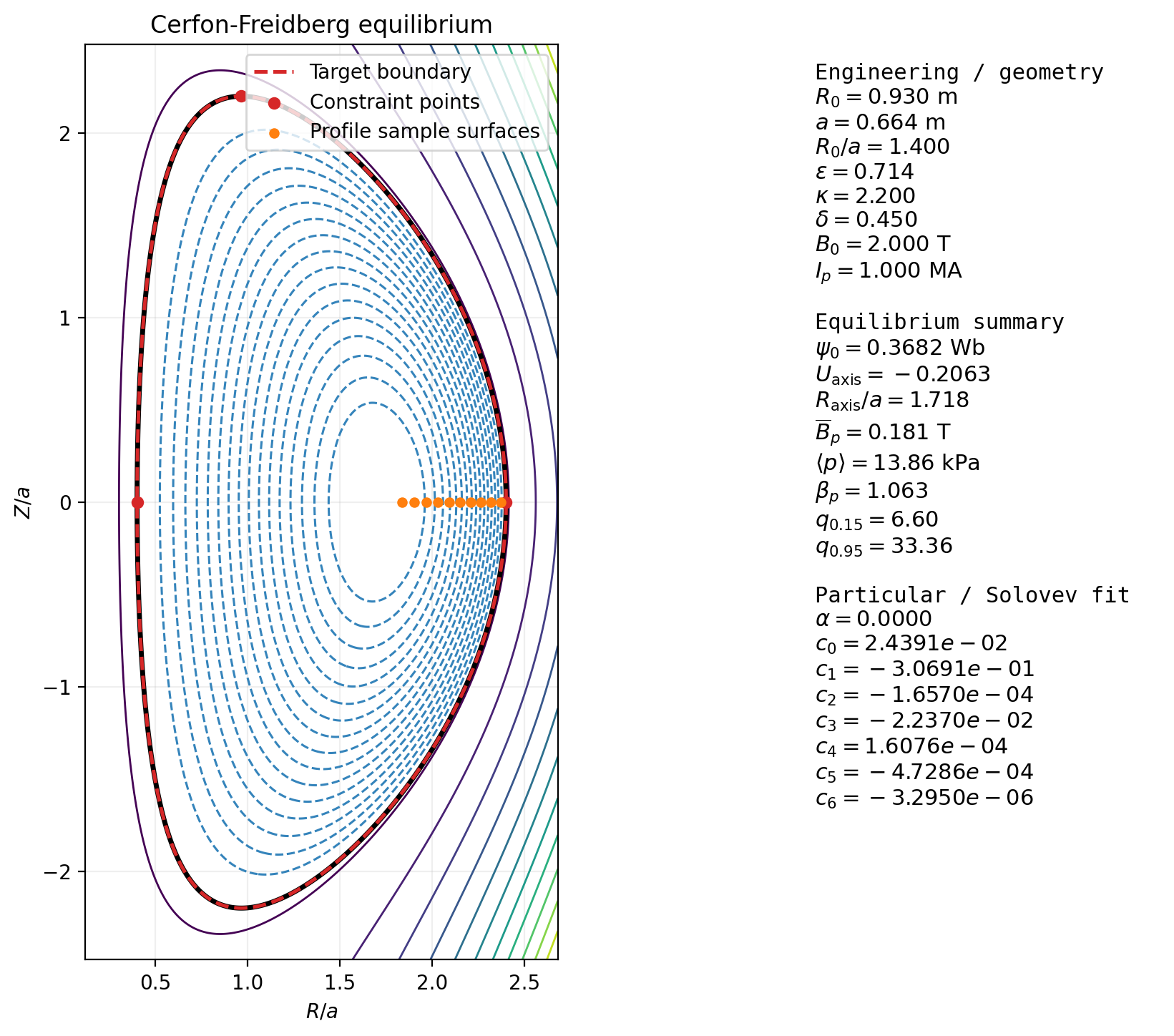
Interactive Cerfon Solver
Open a slider-driven browser explorer for the shaped Solov’ev fit. The app adjusts \(R_0/a\), \(\kappa\), \(\delta\), and the source-mix parameter \(\alpha\), then overlays the target boundary against the fitted \(U=0\) surface and interior flux contours.
Open the equilibrium explorer
Interactive PF-Coil Flux Explorer
Open a browser companion for the external coil set. ITER, SPARC, and DIII-D presets provide simplified central-solenoid, PF-shaping, divertor, vertical-field, and plasma-current contributions, and a checkmark table lets you decide which pieces build the total equilibrium and which single family is being contoured.
Open the coil-flux explorer
Most General Solution
One can extend the Solov’ev technique to include a broader collection of homogeneous solutions that make
creating equilibria with different shapes quite general. Best to first non-dimensionalize and construct a
particular solution. Write
\[R=R_0 X, \qquad Z=R_0 Y, \qquad \psi = \psi _0 U(X,Y),\]
with \(\psi _0 = R_0^2(A+C R_0^2)\). Then Eq. (10.28) becomes \[X\pp {}{X}\!\left (\frac {1}{X}\pp {U}{X}\right ) + \pp {^2 U}{Y^2} = \alpha + (1-\alpha )X^2, \tag{10.45}\]
for a convenient parameter \(\alpha \): \(\alpha = 1 \) being all \(FF'\) and \(\alpha = 0\) being all \(p'\). A particular solution is \[U_p(X,Y) = \frac {\alpha }{2}X^2 \ln X + \frac {1-\alpha }{8}X^4. \tag{10.46}\]
The homogeneous equation \[X\pp {}{X}\!\left (\frac {1}{X}\pp {U_H}{X}\right ) + \pp {^2 U_H}{Y^2} = 0\]
admits polynomial basis functions such as \[\begin {aligned} U_0 &= 1, & U_1 &= X^2, \\ U_2 &= Y^2-X^2\ln X, & U_3 &= X^4-4X^2Y^2, \\ U_4 &= 2Y^4-9X^2Y^2+3X^4\ln X-12X^2Y^2\ln X, & U_5 &= X^6-12X^4Y^2+8X^2Y^4, \\ U_6 &= 8Y^6-140X^2Y^4+75X^4Y^2 -15X^6\ln X \\ & \phantom {=} +180X^4Y^2\ln X -120X^2Y^4\ln X. \end {aligned}\]
Hence one may write \[U(X,Y)=U_p(X,Y)+\sum _{j=0}^{6} c_j U_j(X,Y). \tag{10.49}\]
This family is valuable because it is flexible enough to represent shaped equilibria while still being
analytic.
Why Solov’ev equilibria are still useful.
They are analytically tractable, they expose how shaping enters the flux geometry, and they provide
benchmark solutions for numerical codes. That is why they remain a classic problem in their own right and
continue to appear in analytical work and code verification.
10.5 Dynamic Equilibria: Toroidal Rotation
Allow purely toroidal flow,
\[\uvec = R \Omega (R,Z) \grad \phi .\]
The steady momentum equation becomes
\[\rho (\uvec \cdot \grad ) \uvec = \J \times \B - \grad p . \tag{10.51}\]
Ferraro’s isorotation theorem
Ideal Ohm’s law, \[ \E + \uvec \times \B = 0, \] and \(\pp {\vect {B}}{t}\) implies \[ \curl (\uvec \times \B )=0. \]
For purely rotating plasmas \(\uvec = R^2 \Omega \grad \phi \), and
\[\begin {aligned} \vect {u}\times \vect {B} &= R^2 \Omega \nabla \phi \times \nabla \psi \times \nabla \phi \\ &= \Omega \nabla \psi . \end {aligned}\]
Since \(\nabla \times \Omega \nabla \psi = \nabla \Omega \times \nabla \psi = 0\) it follows that \[\boxed { \Omega = \Omega (\psi ). }\]
Parallel force balance
Projecting (10.51) along \(\B \) gives
\[\frac {\partial p}{\partial \ell } + n m_i \Omega ^2(\psi ) R \frac {\partial R}{\partial \ell } = 0.\]
Assuming \(T=T(\psi )\) and \(p=nT\), this integrates to
\[\boxed { p(\psi ,R) = p_0(\psi ) \exp \!\left [ \frac {\Omega ^2(\psi )}{2 c_s^2(\psi )} (R^2 - R_0^2) \right ]. } \tag{10.55}\]
Modified Grad–Shafranov equation
Because \(p=p(\psi ,R)\),
\[\boxed { \Delta ^\star \psi = -\muo R^2 \pp {}{\psi }p(\psi ,R) - F \pp {F}{\psi }. } \tag{10.56}\]
Rotation modifies equilibrium implicitly through the \(R\)-dependent pressure profile, while Ferraro’s theorem
ensures rigid rotation on each flux surface.
Takeaways
- In isotropic axisymmetric equilibrium, both \(p\) and \(F\) become functions of the flux \(\psi \).
- The Grad–Shafranov equation, Eq. (10.28), is the single PDE that enforces force
balance on flux surfaces.
- Solving the equation requires three choices: a domain, boundary conditions, and the
free functions \(p(\psi )\) and \(F(\psi )\).
- Analytic families such as Solovév equilibria are useful because they show how shaping
enters before one commits to full numerical reconstruction.
Bibliography
V. D. Shafranov. On magnetohydrodynamical equilibrium configurations. Soviet Physics JETP, 6(3):545–554, 1958. English translation of Zh. Eksp. Teor. Fiz. 33, 710–722 (1957).
V. D. Shafranov. Equilibrium of a plasma toroid in a magnetic field. Soviet Physics JETP, 10(4):775–779, 1960. English translation of Zh. Eksp. Teor. Fiz. 37, 1088–1095 (1959).
V. D. Shafranov. Plasma equilibrium in a magnetic field. In M. A. Leontovich, editor, Reviews of Plasma Physics, volume 2, pages 103–151. Consultants Bureau, New York, 1966. Classic long review; includes the large-aspect-ratio treatment used for what is commonly called the Shafranov shift.
Harold Grad. Toroidal containment of a plasma. The Physics of Fluids, 10(1):137–154, 1967. doi:10.1063/1.1761965.
A. J. Cerfon and J. P. Freidberg. One size fits all: Reconstruction of tokamak equilibria with free-boundary grad–shafranov solvers. Physics of Plasmas, 17:032502, 2010.
Problems
Problem 10.1. Derive the Grad–Shafranov equation from scratch
Part A.
Starting from Eq. (10.1), derive Eq. (10.2).
Part B.
Use Eq. (1.11) to derive Eqs. (10.7) and (10.8). Do not skip the algebra that produces the operator
\(\Delta ^\star \).
Part C.
Starting from Eq. (10.10), show that \(p=p(\psi )\) and \(F=F(\psi )\).
Part D.
Reproduce Eqs. (10.22) and (10.24), and hence derive Eq. (10.28).
Problem 10.2. Solovév equilibria and Green’s functions
Part A.
Verify Eq. (10.37) directly by acting with \(\Delta ^\star \) on \(R^4\), \(Z^2\), and \(R^4-4R^2Z^2\).
Part B.
Starting from Eq. (10.35), derive the particular solution Eq. (10.40) and then verify the full family
Eq. (10.42).
Part C.
For a toroidal current filament located at \((R_{\rm coil},Z_{\rm coil})\), derive the Green’s-function expression leading to Eq. (12.48).
Show where the complete elliptic integrals enter.
Part D.
Implement a simple code to plot contours of \(\psi \) for a dipole, quadrupole, and octupole arrangement of
external coils, following the configurations described in the figure-caption discussion.