Lecture 35
Kinetic examples for \(p_\perp (\psi ,B)\) and \(p_\parallel (\psi ,B)\)
Overview
This appendix gives four explicit kinetic realizations of the functions \(p_\perp (\psi ,B)\) and \(p_\parallel (\psi ,B)\) used in the
anisotropic-equilibrium lectures. The point is not that these are the only useful closures.
The point is that they make the local magnetic-field dependence completely concrete.
Once a guiding-center distribution is written in terms of the invariants \((\psi ,E,\mu )\), the dependence
of the moments on the local field strength \(B\) can be computed directly.
The four examples are:
-
1.
- a fixed-pitch “sloshing-ion” distribution, appropriate to an idealized NBI population;
-
2.
- a regularized fixed-pitch/slowing-down model built from a finite midplane pitch
spread;
-
3.
- the logarithmic mirror distribution obtained from the Lorentz pitch-angle-scattering
operator;
-
4.
- the isotropic Maxwellian limit, for which the pressure is independent of \(B\).
Historical Perspective
These examples sit at the meeting point of two classic lines of thought. One is
mirror-machine kinetics, where trapping, turning points, and pitch-angle scattering
naturally produce anisotropic pressures. The other is anisotropic MHD equilibrium
theory, where one wants to know not merely that \(p_\perp \neq p_\parallel \), but how those quantities vary along
a field line. The cleanest bridge between the two is to compute the velocity moments of
simple distributions written in the adiabatic invariants \((E,\mu )\).
Caution
This appendix is about kinetic realizations of equilibrium moments, not about a full
transport or Fokker–Planck solve. The formulas below are therefore best read as
analytically transparent models that show how a chosen pitch-angle structure maps into
\(p_\perp (\psi ,B)\) and \(p_\parallel (\psi ,B)\).
Throughout this appendix, \(T\) is measured in energy units, so that a Maxwellian factor is written as
\(\exp (-E/T)\). We also assume that the distribution is even in \(v_\parallel \), unless explicitly stated otherwise. This
means that both signs of the parallel velocity are included in the kinetic moments. Relative
to some one-sided slide conventions, this changes only overall numerical prefactors, not the
\(B\)-dependence.
Strategy.
Every example follows the same pattern:
-
1.
- write the distribution in the invariants \((\psi ,E,\mu )\) or \((v,\xi )\);
-
2.
- evaluate the density and pressure moments;
-
3.
- read off the resulting functions \(p_\perp (\psi ,B)\) and \(p_\parallel (\psi ,B)\).
The basic kinematics are common to all four examples, so we begin there.
35.1 General moment formulas in \((E,\mu )\) coordinates
Define
\[E \equiv \frac {m}{2}\left (v_\parallel ^2+v_\perp ^2\right ), \qquad \mu \equiv \frac {m v_\perp ^2}{2B}, \qquad \xi \equiv \frac {v_\parallel }{v}. \tag{C.1}\]
Then \[v_\perp ^2 = \frac {2\mu B}{m}, \qquad |v_\parallel | = \sqrt {\frac {2}{m}\bigl (E-\mu B\bigr )}. \tag{C.2}\]
The inequality \(E-\mu B\ge 0\) is the local accessibility condition: at a point where the field strength is \(B\), only particles
with enough parallel energy can be present.
Tutorial
Why the local field strength enters the moments. If the distribution is written as \(f=f(\psi ,E,\mu )\), then
it has no explicit dependence on the local magnetic field other than through the kinematic
relation \(v_\parallel ^2 = 2(E-\mu B)/m\). This dependence appears in two places only:
-
1.
- in the Jacobian for the transformation from velocity space to \((E,\mu )\), and
-
2.
- in the upper integration limit \(\mu \le E/B\), which enforces \(E-\mu B\ge 0\).
This is the entire origin of the \(B\)-dependence of \(n\), \(p_\perp \), and \(p_\parallel \) in the kinetic examples
below.
Starting from \[ d^3v = 2\pi v_\perp \,dv_\perp \,dv_\parallel , \] and using the fact that the distribution is even in \(v_\parallel \), we may integrate over \(|v_\parallel |\ge 0\) and include both
signs at once: \[ d^3v = 4\pi v_\perp \,dv_\perp \,d|v_\parallel |. \] Now treat \((v_\perp ,|v_\parallel |)\) as functions of \((\mu ,E)\). From \[ E = \frac {m}{2}\left (v_\parallel ^2+v_\perp ^2\right ), \qquad \mu = \frac {m v_\perp ^2}{2B}, \] one finds \[ \frac {\partial (E,\mu )}{\partial (v_\perp ,|v_\parallel |)} = \begin {vmatrix} m v_\perp & m |v_\parallel | \\ \dfrac {m v_\perp }{B} & 0 \end {vmatrix} = -\frac {m^2 v_\perp |v_\parallel |}{B}. \] Therefore
\[dv_\perp \,d|v_\parallel | = \frac {B}{m^2 v_\perp |v_\parallel |}\,dE\,d\mu ,\]
and hence \[d^3v = \frac {4\pi B}{m^2 |v_\parallel |}\,dE\,d\mu = \frac {2\sqrt {2}\pi B}{m^{3/2}} \frac {dE\,d\mu }{\sqrt {E-\mu B}}. \tag{C.4}\]
With the standard gyrotropic definitions
\[n = \int f\,d^3v, \qquad p_\parallel = m\int v_\parallel ^2 f\,d^3v, \qquad p_\perp = \frac {m}{2}\int v_\perp ^2 f\,d^3v, \tag{C.5}\]
Eqs. (C.2)–(C.4) give \[\begin{aligned}n(\psi ,B) &= \frac {2\sqrt {2}\pi B}{m^{3/2}} \int _0^\infty dE \int _0^{E/B} \frac {f(\psi ,E,\mu )}{\sqrt {E-\mu B}}\,d\mu , \\[0.5em] p_\perp (\psi ,B) &= \frac {2\sqrt {2}\pi B^2}{m^{3/2}} \int _0^\infty dE \int _0^{E/B} \frac {\mu \,f(\psi ,E,\mu )}{\sqrt {E-\mu B}}\,d\mu , \\[0.5em] p_\parallel (\psi ,B) &= \frac {4\sqrt {2}\pi B}{m^{3/2}} \int _0^\infty dE \int _0^{E/B} \sqrt {E-\mu B}\,f(\psi ,E,\mu )\,d\mu .\end{aligned} \tag{C.6}\]
The upper limit \(\mu =E/B\) is simply the statement that the local parallel energy \(E-\mu B\) must be non-negative.
A useful identity.
If the distribution is written in adiabatic variables as \(f=f(\psi ,E,\mu )\), with no explicit dependence on the local field
strength beyond the kinematic limit \(\mu \le E/B\), then the equilibrium identity derived in the main lecture
follows directly from the moments above. Differentiate Eq. (C.8) with respect to \(B\) at fixed \(\psi \):
\[\begin{aligned}\frac {\partial p_\parallel }{\partial B} &= \frac {p_\parallel }{B} + \frac {4\sqrt {2}\pi B}{m^{3/2}} \int _0^\infty dE\, \frac {\partial }{\partial B} \int _0^{E/B} \sqrt {E-\mu B}\,f\,d\mu .\end{aligned}\]
Using Leibniz’ rule,
\[\begin{aligned}\frac {\partial }{\partial B} \int _0^{E/B} \sqrt {E-\mu B}\,f\,d\mu &= \int _0^{E/B} \frac {\partial }{\partial B}\Bigl (\sqrt {E-\mu B}\Bigr )f\,d\mu + \left .\frac {d(E/B)}{dB}\sqrt {E-\mu B}\,f\right |_{\mu =E/B}.\end{aligned}\]
The boundary term vanishes because \(\sqrt {E-\mu B}=0\) at \(\mu =E/B\). Therefore
\[\begin{aligned}\frac {\partial p_\parallel }{\partial B} &= \frac {p_\parallel }{B} - \frac {2\sqrt {2}\pi B}{m^{3/2}} \int _0^\infty dE \int _0^{E/B} \frac {\mu f}{\sqrt {E-\mu B}}\,d\mu \\ &= \frac {p_\parallel -p_\perp }{B}.\end{aligned}\]
Hence
\[\boxed { p_\perp = p_\parallel - B\left .\frac {\partial p_\parallel }{\partial B}\right |_{\psi }. } \tag{C.13}\]
This is exactly the \(p_\perp (\psi ,B)\)–\(p_\parallel (\psi ,B)\) relation needed in the equilibrium lecture. The point is worth emphasizing: it is
not merely a fluid closure assumption. It follows directly from any distribution of the form
\(f(\psi ,E,\mu )\).
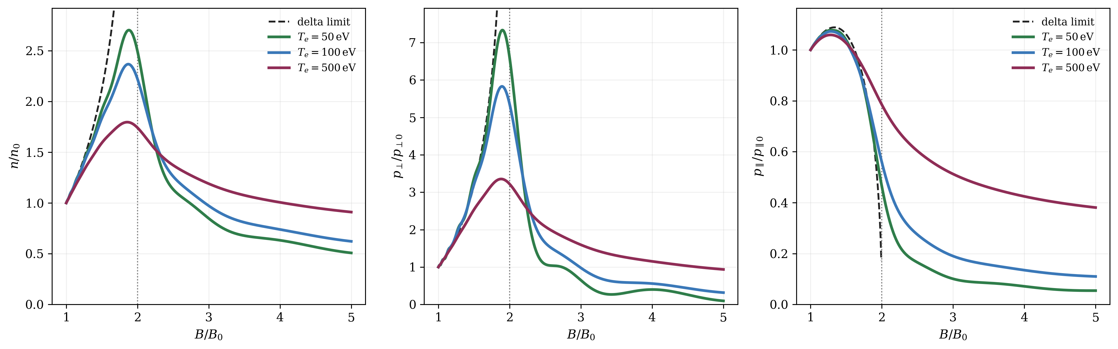
35.2 Fixed-pitch sloshing ions
A simple model for an idealized sloshing-ion population is that the pitch angle at the midplane remains
fixed while the ions slow down. Let \(B_0(\psi )\) be the midplane field on a flux surface and let \(B_T(\psi )\) be the turning-point
field associated with the injected pitch angle. Then
\[\sin ^2\theta _0 = \frac {B_0}{B_T}, \qquad \frac {\mu }{E} = \frac {1}{B_T}. \tag{C.14}\]
A convenient invariant form for the distribution is \[f_{\rm sl}(\psi ,E,\mu ) = C_{\rm sl}(\psi )\,g(E) \,\delta \!\left (\mu -\frac {E}{B_T}\right ). \tag{C.15}\]
The original Bilikman–Mirnov sloshing-ion model corresponds to a slowing-down envelope \(g(E)\propto E^{-3/2}\) between
injection and cutoff energies; however, the \(B\)-dependence derived below does not depend on the detailed
choice of \(g(E)\).
Substitute Eq. (C.15) into Eq. (C.6):
\[\begin{aligned}n(\psi ,B) &= \frac {2\sqrt {2}\pi C_{\rm sl} B}{m^{3/2}} \int _0^\infty dE \int _0^{E/B} \frac {g(E)\,\delta \!\left (\mu -E/B_T\right )}{\sqrt {E-\mu B}}\,d\mu .\end{aligned}\]
For \(B<B_T\), the delta function lies inside the integration range, so
\[n(\psi ,B) = \frac {2\sqrt {2}\pi C_{\rm sl} B}{m^{3/2}} \frac {1}{\sqrt {1-B/B_T}} \int _0^\infty \frac {g(E)}{\sqrt {E}}\,dE. \tag{C.17}\]
Likewise, \[\begin{aligned}p_\perp (\psi ,B) &= \frac {2\sqrt {2}\pi C_{\rm sl} B^2}{m^{3/2}} \int _0^\infty dE \int _0^{E/B} \frac {\mu \,g(E)\,\delta \!\left (\mu -E/B_T\right )}{\sqrt {E-\mu B}}\,d\mu \\ &= \frac {2\sqrt {2}\pi C_{\rm sl} B^2}{m^{3/2} B_T} \frac {1}{\sqrt {1-B/B_T}} \int _0^\infty \sqrt {E}\,g(E)\,dE, \\[0.5em] p_\parallel (\psi ,B) &= \frac {4\sqrt {2}\pi C_{\rm sl} B}{m^{3/2}} \int _0^\infty dE \int _0^{E/B} \sqrt {E-\mu B}\,g(E)\,\delta \!\left (\mu -E/B_T\right )d\mu \\ &= \frac {4\sqrt {2}\pi C_{\rm sl} B}{m^{3/2}} \sqrt {1-B/B_T} \int _0^\infty \sqrt {E}\,g(E)\,dE.\end{aligned} \tag{C.19}\]
It is often cleaner to normalize these profiles to their midplane values, defined at \(B=B_0\):
\[\begin{aligned}\frac {n(\psi ,B)}{n_0(\psi )} &= \frac {B}{B_0} \sqrt {\frac {1-B_0/B_T}{1-B/B_T}}, \\[0.5em] \frac {p_\perp (\psi ,B)}{p_{\perp 0}(\psi )} &= \frac {B^2}{B_0^2} \sqrt {\frac {1-B_0/B_T}{1-B/B_T}}, \\[0.5em] \frac {p_\parallel (\psi ,B)}{p_{\parallel 0}(\psi )} &= \frac {B}{B_0} \sqrt {\frac {1-B/B_T}{1-B_0/B_T}}.\end{aligned} \tag{C.22}\]
These are the fixed-pitch sloshing-ion profiles in the form most convenient for equilibrium
work.
Caution
Turning-point singularity. As \(B\to B_T\),
\[n,\ p_\perp \propto \frac {1}{\sqrt {1-B/B_T}}, \qquad p_\parallel \propto \sqrt {1-B/B_T}. \tag{C.25}\]
So the strict delta-function pitch-angle model produces the familiar turning-point singularity in
\(n\) and \(p_\perp \). A small but finite angular spread regularizes this divergence. The fixed-pitch model is
therefore best regarded as an analytically useful limiting case. Section C.3 shows how the
singularity is removed by replacing the delta-function pitch distribution by a finite-width
midplane kernel.
If the energy envelope is Maxwellian.
For
\[g(E)=g_0 e^{-E/T}, \tag{C.26}\]
one may evaluate the energy integrals explicitly: \[\int _0^\infty E^{-1/2}e^{-E/T}\,dE = \sqrt {\pi T}, \qquad \int _0^\infty E^{1/2}e^{-E/T}\,dE = \frac {\sqrt {\pi }}{2}T^{3/2}. \tag{C.27}\]
Hence Eqs. (C.17)–(C.21) reduce to the same \(B\)-dependences as above, now with explicit amplitudes
proportional to \(\sqrt {T}\) and \(T^{3/2}\).
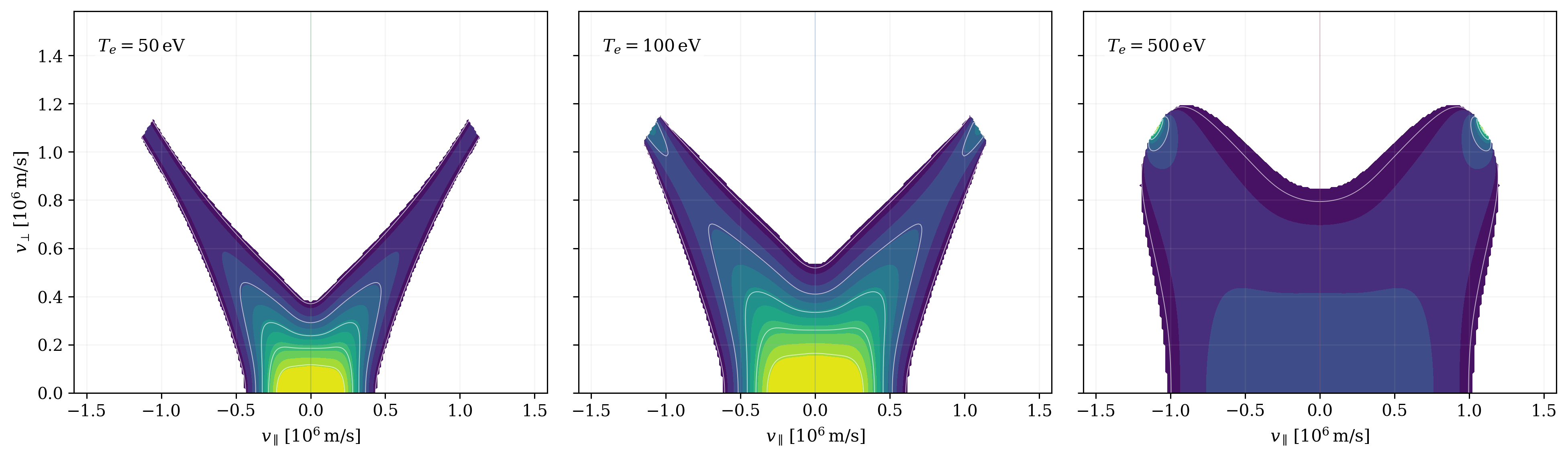
35.3 A regularized fixed-pitch model from the fast-ion Fokker–Planck equation
The strict fixed-pitch model of the previous section is the singular limit of a more realistic construction in
which the midplane pitch variable has a small but finite width. For neutral-beam ions this width should
increase as the ions slow down and scatter. A convenient way to organize the calculation is to start from
the fast-ion Fokker–Planck equation, then rewrite the resulting midplane distribution in terms of the
invariant pitch variable
\[\lambda \equiv \frac {\mu B_0}{E} = \sin ^2\theta _0 = 1-\xi _0^2, \qquad \xi _0 \equiv \frac {v_{\parallel ,0}}{v_0}, \qquad B_0 \equiv B_{\rm midplane}(\psi ). \tag{C.28}\]
Here \(\xi _0\) is the injected midplane pitch cosine and \(\lambda \) labels the turning-point field through \[B_T = \frac {B_0}{\lambda }, \qquad \lambda _0 = \frac {B_0}{B_T} = 1-\xi _0^2. \tag{C.29}\]
Thus the delta-function fixed-pitch model is simply the limit in which all particles sit at one value
\(\lambda =\lambda _0\).
Fast-ion Fokker–Planck equation.
Following Callen’s treatment of a fast beam injected into a Maxwellian background, and neglecting the
small initial speed-diffusion layer, the fast-ion distribution \(f_f(v,\zeta ,t)\) obeys
\[\tau _s\,\partial _t f_f = \frac {m_i v_c^3}{2m_f v^3} \frac {\partial }{\partial \zeta } \left [(1-\zeta ^2)\frac {\partial f_f}{\partial \zeta }\right ] + \frac {1}{v^2}\frac {\partial }{\partial v}\left [(v^3+v_c^3)f_f\right ] + \frac {\dot n_f\tau _s}{2\pi v_0^2} \delta (v-v_0)\,\delta (\zeta -\zeta _0)\,H(t). \tag{C.30}\]
Here \(m_f\) is the fast-ion mass, \(m_i\) is the background ion mass, \(\tau _s\) is the electron-drag slowing-down time, \(v_c\) is the
critical speed, \(\dot n_f\) is the source rate, and \(\zeta \equiv v_\parallel /v\). The source is a delta-function beam injected at speed \(v_0\) and pitch
cosine \(\zeta _0\), which we identify with the midplane injection angle, \[\zeta _0 = \xi _0. \tag{C.31}\]
The first term on the right-hand side of Eq. (C.30) is pitch-angle scattering, while the second term is the
slowing-down drift in speed.
Callen’s series solution.
Expanding in Legendre polynomials gives the explicit solution
\[\boxed { f_f(v,\zeta ,t) = \frac {\dot n_f\tau _s}{2\pi \,(v^3+v_c^3)} \sum _{l=0}^{\infty } \left (l+\frac 12\right ) P_l(\zeta )P_l(\zeta _0) W_l(v) H\!\left [t-\tau (v)\right ]H(v_0-v), } \tag{C.32}\]
with \[W_l(v) = \left [ \frac {v^3}{v_0^3} \frac {v_0^3+v_c^3}{v^3+v_c^3} \right ]^{\frac {m_i}{6m_f}l(l+1)}, \qquad \tau (v) = \frac {\tau _s}{3} \ln \!\left (\frac {v_0^3+v_c^3}{v^3+v_c^3}\right ). \tag{C.33}\]
For \(v\gg v_c\), the angular distribution remains narrowly concentrated around the injected pitch. As the ions slow
through \(v\sim v_c\), the factors \(W_l(v)\) strongly damp the higher Legendre modes, producing the desired pitch
broadening.
Even part relevant for pressure moments.
The density and pressure moments depend only on the part of the distribution that is even in \(v_\parallel \), so it is
convenient to define
\[f_f^{(+)}(v,\zeta ,t) \equiv \frac 12\left [f_f(v,\zeta ,t)+f_f(v,-\zeta ,t)\right ]. \tag{C.34}\]
Using \(P_l(-\zeta )=(-1)^lP_l(\zeta )\), only even Legendre harmonics survive: \[f_f^{(+)}(v,\zeta ,t) = \frac {\dot n_f\tau _s}{2\pi \,(v^3+v_c^3)} \sum _{j=0}^{\infty } \frac {4j+1}{2} P_{2j}(\zeta )P_{2j}(\xi _0) W_{2j}(v) H\!\left [t-\tau (v)\right ]H(v_0-v). \tag{C.35}\]
Midplane pitch density in \(\lambda \).
For equilibrium work it is natural to convert from \(\mu \) to the midplane pitch variable \(\lambda =\mu B_0/E\). Define the midplane
pitch density \(F_0\) by
\[F_0(\psi ,E,\lambda ,t)\,d\lambda \equiv f(\psi ,E,\mu ,t)\,d\mu , \qquad \mu = \frac {E\lambda }{B_0}, \tag{C.36}\]
so that \[F_0(\psi ,E,\lambda ,t) = \frac {E}{B_0} f\!\left (\psi ,E,\mu =\frac {E\lambda }{B_0},t\right ). \tag{C.37}\]
At the midplane, \(\lambda =1-\zeta ^2\), and therefore the Callen solution induces \[\boxed { F_0^{\rm Callen}(\psi ,E,\lambda ,t) = \frac {E}{B_0} f_f^{(+)}\!\left (v(E),\sqrt {1-\lambda },t\right ), \qquad v(E)=\sqrt {\frac {2E}{m_f}}. } \tag{C.38}\]
Substituting Eq. (C.35) gives \[\begin{aligned}F_0^{\rm Callen}(\psi ,E,\lambda ,t) &= \frac {E}{B_0} \frac {\dot n_f\tau _s}{2\pi \,[v(E)^3+v_c^3]} \sum _{j=0}^{\infty } \frac {4j+1}{2} P_{2j}(\sqrt {1-\lambda })P_{2j}(\xi _0) W_{2j}(E) \notag \\ &\qquad \times H\!\left [t-\tau (E)\right ]H(E_0-E),\end{aligned} \tag{C.39}\]
where
\[E_0 \equiv \frac 12 m_f v_0^2, \qquad E_c \equiv \frac 12 m_f v_c^2, \tag{C.40}\]
\[W_l(E) = \left [ \left (\frac {E}{E_0}\right )^{3/2} \frac {E_0^{3/2}+E_c^{3/2}}{E^{3/2}+E_c^{3/2}} \right ]^{\frac {m_i}{6m_f}l(l+1)}, \qquad \tau (E) = \frac {\tau _s}{3} \ln \!\left (\frac {E_0^{3/2}+E_c^{3/2}}{E^{3/2}+E_c^{3/2}}\right ). \tag{C.41}\]
At late times after the beam has populated the accessible slowing-down interval, one may simply set \(H[t-\tau (E)]\to 1\) for
the occupied energies.
Moment formulas in \((E,\lambda )\) form.
Now let
\[b \equiv \frac {B}{B_0}. \tag{C.42}\]
Since \[E-\mu B = E(1-b\lambda ), \qquad \mu = \frac {E\lambda }{B_0}, \qquad d\mu = \frac {E}{B_0}\,d\lambda , \tag{C.43}\]
Eqs. (C.6)–(C.8) become \[\begin{aligned}n(\psi ,B) &= \frac {2\sqrt {2}\pi B_0 b}{m_f^{3/2}} \int _0^\infty \frac {dE}{\sqrt {E}} \int _0^{1/b} \frac {F_0(\psi ,E,\lambda )}{\sqrt {1-b\lambda }}\,d\lambda , \\ p_\perp (\psi ,B) &= \frac {2\sqrt {2}\pi B_0 b^2}{m_f^{3/2}} \int _0^\infty \sqrt {E}\,dE \int _0^{1/b} \frac {\lambda \,F_0(\psi ,E,\lambda )}{\sqrt {1-b\lambda }}\,d\lambda , \\ p_\parallel (\psi ,B) &= \frac {4\sqrt {2}\pi B_0 b}{m_f^{3/2}} \int _0^\infty \sqrt {E}\,dE \int _0^{1/b} \sqrt {1-b\lambda }\,F_0(\psi ,E,\lambda )\,d\lambda .\end{aligned} \tag{C.44}\]
The upper limit \(\lambda \le 1/b\) is just the local accessibility condition. If only mirror-trapped particles are desired on a
field line with maximum field \(B_{\max }\), one may further restrict the support to \(\lambda \ge B_0/B_{\max }\).
Delta-function fixed-pitch limit in midplane variables.
The strict fixed-pitch model is recovered by taking
\[F_0^{(\delta )}(\psi ,E,\lambda ) = C_{\rm sl}(\psi )\,g(E)\,\delta (\lambda -\lambda _0), \qquad \lambda _0 = 1-\xi _0^2 = \frac {B_0}{B_T}. \tag{C.47}\]
Substitution into Eqs. (C.44)–(C.46) gives \[\begin{aligned}\frac {n(\psi ,B)}{n_0(\psi )} &= b\sqrt {\frac {1-\lambda _0}{1-b\lambda _0}}, \\[0.5em] \frac {p_\perp (\psi ,B)}{p_{\perp 0}(\psi )} &= b^2\sqrt {\frac {1-\lambda _0}{1-b\lambda _0}} = b^2\frac {|\xi _0|}{\sqrt {1-b(1-\xi _0^2)}}, \\[0.5em] \frac {p_\parallel (\psi ,B)}{p_{\parallel 0}(\psi )} &= b\sqrt {\frac {1-b\lambda _0}{1-\lambda _0}} = b\frac {\sqrt {1-b(1-\xi _0^2)}}{|\xi _0|}.\end{aligned} \tag{C.48}\]
These are the previous fixed-pitch profiles rewritten directly in terms of the injection angle. The singularity
occurs at the turning field \(b=1/\lambda _0\).
Generic finite-width regularization.
A mathematically clean regularization is obtained by replacing the delta function by a normalized kernel,
\[F_0(\psi ,E,\lambda ) = C_{\rm sl}(\psi )\,g(E) K\!\left (\lambda ;\lambda _0,\sigma _\lambda (E)\right ), \qquad \int _0^1 K\!\left (\lambda ;\lambda _0,\sigma _\lambda \right )d\lambda =1. \tag{C.51}\]
Then \[\begin{aligned}p_\perp (\psi ,B) &= \frac {2\sqrt {2}\pi B_0 b^2 C_{\rm sl}}{m_f^{3/2}} \int _0^\infty \sqrt {E}\,g(E) \left [ \int _0^{1/b} \frac {\lambda \,K(\lambda ;\lambda _0,\sigma _\lambda (E))}{\sqrt {1-b\lambda }}\,d\lambda \right ]dE, \\ p_\parallel (\psi ,B) &= \frac {4\sqrt {2}\pi B_0 b C_{\rm sl}}{m_f^{3/2}} \int _0^\infty \sqrt {E}\,g(E) \left [ \int _0^{1/b} \sqrt {1-b\lambda } K(\lambda ;\lambda _0,\sigma _\lambda (E))\,d\lambda \right ]dE.\end{aligned} \tag{C.52}\]
Because the endpoint singularity \(\int ^{1/b}d\lambda /\sqrt {1-b\lambda }\) is integrable, any finite-width kernel removes the fixed-pitch
divergence.
A positive kernel approximation extracted from Callen’s solution.
The exact series solution in Eq. (C.39) need not be evaluated term by term if one only wants a narrow
positive kernel with the correct first few pitch moments. At fixed energy,
\[\langle P_2(\zeta )\rangle _E = P_2(\xi _0)W_2(E), \qquad \langle P_4(\zeta )\rangle _E = P_4(\xi _0)W_4(E). \tag{C.54}\]
Using \[P_2(\zeta )=\frac 12(3\zeta ^2-1), \qquad P_4(\zeta )=\frac 18(35\zeta ^4-30\zeta ^2+3), \tag{C.55}\]
one obtains \[\langle \zeta ^2\rangle _E = \frac {1+2P_2(\xi _0)W_2(E)}{3}, \tag{C.56}\]
\[\langle \zeta ^4\rangle _E = \frac {7+20P_2(\xi _0)W_2(E)+8P_4(\xi _0)W_4(E)}{35}. \tag{C.57}\]
Therefore an energy-dependent Gaussian kernel in \(\lambda =1-\zeta ^2\) may be built from \[\bar \lambda (E) = 1-\langle \zeta ^2\rangle _E, \qquad \sigma _\lambda ^2(E) = \langle \zeta ^4\rangle _E-\langle \zeta ^2\rangle _E^2, \tag{C.58}\]
and \[K_G(\lambda ;E) = \frac {\exp \!\left [-(\lambda -\bar \lambda (E))^2/2\sigma _\lambda ^2(E)\right ]} {\int _0^1 \exp \!\left [-(\lambda -\bar \lambda (E))^2/2\sigma _\lambda ^2(E)\right ]d\lambda }, \qquad 0\le \lambda \le 1. \tag{C.59}\]
This replaces the singular delta-function pitch model by a positive, energy-dependent kernel whose width
automatically increases as the beam slows toward \(v_c\).
Implementation formulas for \(v_0\), \(v_c\), \(E_c\), and \(\tau _s\).
For computer implementation, it is convenient to begin from the injected fast-ion energy \(E_{\rm inj}\) and the injected
pitch angle \(\theta _{\rm inj}\) at the midplane:
\[E_0 = e\,E_{\rm inj}[\mathrm {eV}], \qquad T_e = e\,T_e[\mathrm {eV}], \qquad \xi _0 = \cos \theta _{\rm inj}, \qquad \lambda _0 = 1-\xi _0^2. \tag{C.60}\]
Then \[v_0 = \sqrt {\frac {2E_0}{m_f}}. \tag{C.61}\]
The background-electron thermal speed is \[v_{the} = \sqrt {\frac {2T_e}{m_e}}, \tag{C.62}\]
and the critical speed is \[v_c = \left [\frac {3\sqrt {\pi }}{4}\frac {m_e}{m_i}\right ]^{1/3}v_{the}. \tag{C.63}\]
Equivalently, \[E_c = \frac 12 m_f v_c^2 = \left [\frac {3\sqrt {\pi }}{4}\sqrt {\frac {m_f}{m_e}}\frac {m_f}{m_i}\right ]^{2/3}T_e. \tag{C.64}\]
In SI units the slowing-down time is
\[\tau _s = \frac {m_f}{m_e} \frac {3(4\pi \epsilon _0)^2\sqrt {m_e}\,T_e^{3/2}} {4\sqrt {2\pi }\,n_e Z_f^2 e^4\ln \Lambda }. \tag{C.65}\]
Thus \(\tau _s\) requires, in addition to \(T_e\), the electron density \(n_e\), the fast-ion charge state \(Z_f\), and the Coulomb logarithm
\(\ln \Lambda \). The slowing-down law may be written either as \[\frac {dv}{dt} = -\frac {v}{\tau _s} \left [1+\left (\frac {v_c}{v}\right )^3\right ], \tag{C.66}\]
or, in energy form, \[\frac {dE}{dt} = -\frac {2E}{\tau _s} \left [1+\left (\frac {E_c}{E}\right )^{3/2}\right ]. \tag{C.67}\]
Its integrated solution is \[t = \frac {\tau _s}{3} \ln \!\left (\frac {v_0^3+v_c^3}{v^3+v_c^3}\right ) = \frac {\tau _s}{3} \ln \!\left (\frac {E_0^{3/2}+E_c^{3/2}}{E^{3/2}+E_c^{3/2}}\right ). \tag{C.68}\]
These are the formulas needed to build either the full Callen series model, Eq. (C.39), or its finite-width
kernel approximation, Eq. (C.59), and then evaluate \(p_\perp (\psi ,B)\) and \(p_\parallel (\psi ,B)\) from Eqs. (C.44)–(C.46).
35.4 The mirror distribution from the Lorentz pitch-angle operator
The logarithmic mirror distribution follows from the simplest collision operator that retains pitch-angle
scattering,
\[C(f)=\nu (E)\,\mathcal {L}f, \qquad \mathcal {L} = \frac {1}{\sin \theta }\frac {\partial }{\partial \theta } \left (\sin \theta \frac {\partial }{\partial \theta }\right ) = \frac {1}{2}\frac {\partial }{\partial \xi } \left [(1-\xi ^2)\frac {\partial }{\partial \xi }\right ], \tag{C.69}\]
with \(\xi =\cos \theta =v_\parallel /v\).
Assume a steady, pitch-angle-independent source at fixed energy,
\[0 = C(f)+S(E) = \frac {\nu (E)}{2}\frac {\partial }{\partial \xi } \left [(1-\xi ^2)\frac {\partial f}{\partial \xi }\right ] + S(E). \tag{C.70}\]
We solve this on the trapped interval \(|\xi |<\xi _T\), where \(\xi _T\) is the local loss-cone boundary. The boundary conditions are
\[f(E,\xi _T)=0, \qquad \left .\frac {\partial f}{\partial \xi }\right |_{\xi =0}=0. \tag{C.71}\]
The second condition expresses symmetry between \(+v_\parallel \) and \(-v_\parallel \).
Integrating Eq. (C.70) once gives
\[(1-\xi ^2)\frac {\partial f}{\partial \xi } = -\frac {2S(E)}{\nu (E)}\xi + C_1(E). \tag{C.72}\]
The symmetry condition at \(\xi =0\) sets \(C_1(E)=0\), so \[\frac {\partial f}{\partial \xi } = -\frac {2S(E)}{\nu (E)}\frac {\xi }{1-\xi ^2}. \tag{C.73}\]
Integrating again, \[f(E,\xi ) = \frac {S(E)}{\nu (E)}\ln (1-\xi ^2)+C_2(E). \tag{C.74}\]
Now use the absorbing boundary condition at \(\xi =\xi _T\): \[0 = \frac {S(E)}{\nu (E)}\ln (1-\xi _T^2)+C_2(E),\]
so that \[\boxed { f_{\rm mir}(E,\xi ) = \frac {S(E)}{\nu (E)} \ln \!\left (\frac {1-\xi ^2}{1-\xi _T^2}\right ), \qquad |\xi |<\xi _T. } \tag{C.76}\]
This is the logarithmic mirror distribution used on the slides.
The same solution gives the classical mirror confinement time.
If the source is uniform in \(\xi \) over \(|\xi |<\xi _c\), then the particle content is proportional to
\[N \propto 2\int _0^{\xi _c} f\,d\xi = \frac {2S}{\nu }\int _0^{\xi _c} \ln \!\left (\frac {1-\xi ^2}{1-\xi _c^2}\right )d\xi ,\]
while the source rate is proportional to \(2\xi _c S\). Therefore \[\tau _p = \frac {1}{\nu \xi _c} \int _0^{\xi _c} \ln \!\left (\frac {1-\xi ^2}{1-\xi _c^2}\right )d\xi . \tag{C.78}\]
Using \[\int \ln (1-\xi ^2)\,d\xi = \xi \ln (1-\xi ^2)-2\xi +\ln \!\left (\frac {1+\xi }{1-\xi }\right ), \tag{C.79}\]
one finds \[\boxed { \tau _p = \frac {1}{\nu \,\xi _c} \left [ \ln \!\left (\frac {1+\xi _c}{1-\xi _c}\right )-2\xi _c \right ]. } \tag{C.80}\]
For a square-well mirror with \(\xi _c^2 = 1-1/R_M\), \[\xi _c \simeq 1-\frac {1}{2R_M}, \qquad R_M\gg 1,\]
and thus \[\tau _p \simeq \frac {1}{\nu }\left (\ln R_M - 0.62\right ). \tag{C.82}\]
This is the standard classical mirror scaling obtained from the Lorentz pitch-angle-scattering
operator.
Rewrite the logarithmic solution in invariant form.
At a given point along a field line,
\[1-\xi ^2 = \frac {\mu B}{E}. \tag{C.83}\]
For particles that turn where the field reaches \(B_T\), the trapped-particle boundary is \[\xi _T^2(B) = 1-\frac {B}{B_T}, \qquad 1-\xi _T^2 = \frac {B}{B_T}. \tag{C.84}\]
Therefore Eq. (C.76) can be rewritten as \[\ln \!\left (\frac {1-\xi ^2}{1-\xi _T^2}\right ) = \ln \!\left (\frac {\mu B/E}{B/B_T}\right ) = \ln \!\left (\frac {\mu B_T}{E}\right ). \tag{C.85}\]
That is, the same mirror distribution can be written as \[f_{\rm mir}(\psi ,E,\mu ) = A_{\rm mir}(\psi ,E) \ln \!\left (\frac {\mu B_T}{E}\right ), \qquad \frac {E}{B_T}\le \mu \le \frac {E}{B}. \tag{C.86}\]
For analytic pressure profiles it is convenient to take a Maxwellian energy envelope, \[A_{\rm mir}(\psi ,E)=A_M(\psi )e^{-E/T}. \tag{C.87}\]
This is not meant to replace the full energy-space Fokker–Planck solution; it is just the cleanest separable
model for exposing the \(B\)-dependence.
Now compute the moments.
At fixed \(B\), define
\[s(B) \equiv \xi _T(B)=\sqrt {1-B/B_T}, \qquad L(s) \equiv \ln \!\left (\frac {1+s}{1-s}\right ). \tag{C.88}\]
Then Eq. (C.76) becomes \[f_{\rm mir}(v,\xi ;B) = A_M e^{-mv^2/2T} \ln \!\left (\frac {1-\xi ^2}{1-s^2}\right ), \qquad |\xi |<s. \tag{C.89}\]
The moments may be written as \[\begin{aligned}n(B) &= 2\pi A_M \int _0^\infty v^2 e^{-mv^2/2T}\,dv \int _{-s}^{s} \ln \!\left (\frac {1-\xi ^2}{1-s^2}\right )d\xi , \\[0.5em] p_\parallel (B) &= 2\pi m A_M \int _0^\infty v^4 e^{-mv^2/2T}\,dv \int _{-s}^{s} \xi ^2\ln \!\left (\frac {1-\xi ^2}{1-s^2}\right )d\xi , \\[0.5em] p_\perp (B) &= \pi m A_M \int _0^\infty v^4 e^{-mv^2/2T}\,dv \int _{-s}^{s} (1-\xi ^2)\ln \!\left (\frac {1-\xi ^2}{1-s^2}\right )d\xi .\end{aligned} \tag{C.90}\]
The speed integrals are elementary:
\[\int _0^\infty v^2 e^{-mv^2/2T}dv = \frac {\sqrt {\pi }}{4}\left (\frac {2T}{m}\right )^{3/2}, \qquad \int _0^\infty v^4 e^{-mv^2/2T}dv = \frac {3\sqrt {\pi }}{8}\left (\frac {2T}{m}\right )^{5/2}. \tag{C.93}\]
So the problem reduces to three angular integrals.
Density integral.
Define
\[\mathcal {N}(s) \equiv \int _{-s}^{s} \ln \!\left (\frac {1-\xi ^2}{1-s^2}\right )d\xi = 2\int _0^{s}\left [\ln (1-\xi ^2)-\ln (1-s^2)\right ]d\xi . \tag{C.94}\]
Using Eq. (C.79), \[\begin{aligned}\mathcal {N}(s) &= 2\left [ \xi \ln (1-\xi ^2)-2\xi +\ln \!\left (\frac {1+\xi }{1-\xi }\right ) \right ]_0^s -2s\ln (1-s^2) \\ &= 2\ln \!\left (\frac {1+s}{1-s}\right )-4s = 2L-4s.\end{aligned} \tag{C.96}\]
Parallel-pressure integral.
Define
\[\mathcal {P}_\parallel (s) \equiv \int _{-s}^{s} \xi ^2\ln \!\left (\frac {1-\xi ^2}{1-s^2}\right )d\xi . \tag{C.97}\]
An antiderivative is \[\int \xi ^2\ln (1-\xi ^2)\,d\xi = \frac {\xi ^3}{3}\ln (1-\xi ^2) -\frac {2}{9}\xi ^3 -\frac {2}{3}\xi +\frac {1}{3}\ln \!\left (\frac {1+\xi }{1-\xi }\right ). \tag{C.98}\]
Therefore \[\begin{aligned}\mathcal {P}_\parallel (s) &= 2\left [ \frac {\xi ^3}{3}\ln (1-\xi ^2) -\frac {2}{9}\xi ^3 -\frac {2}{3}\xi +\frac {1}{3}\ln \!\left (\frac {1+\xi }{1-\xi }\right ) \right ]_0^s - \frac {2}{3}s^3\ln (1-s^2) \nonumber \\ &= \frac {2}{3}\ln \!\left (\frac {1+s}{1-s}\right ) -\frac {4}{3}s -\frac {4}{9}s^3 \nonumber \\ &= \frac {2}{3}L - \frac {4}{3}s - \frac {4}{9}s^3.\end{aligned} \tag{C.99}\]
Perpendicular-pressure integral.
Define
\[\mathcal {P}_\perp (s) \equiv \int _{-s}^{s} (1-\xi ^2)\ln \!\left (\frac {1-\xi ^2}{1-s^2}\right )d\xi . \tag{C.100}\]
Since \((1-\xi ^2)=1-\xi ^2\), \[\mathcal {P}_\perp (s)=\mathcal {N}(s)-\mathcal {P}_\parallel (s),\]
and thus \[\begin{aligned}\mathcal {P}_\perp (s) &= \left (2L-4s\right )-\left (\frac {2}{3}L-\frac {4}{3}s-\frac {4}{9}s^3\right ) \\ &= \frac {4}{3}L-\frac {8}{3}s+\frac {4}{9}s^3.\end{aligned} \tag{C.103}\]
Substituting Eqs. (C.93), (C.96), (C.99), and (C.103) into Eqs. (C.90)–(C.92) gives
\[\begin{aligned}n(\psi ,B) &= \pi ^{3/2}A_M(\psi ) \left (\frac {2T}{m}\right )^{3/2} \Bigl [L(s)-2s\Bigr ], \\[0.5em] p_\parallel (\psi ,B) &= \pi ^{3/2}A_M(\psi )T \left (\frac {2T}{m}\right )^{3/2} \Bigl [L(s)-2s-\frac {2}{3}s^3\Bigr ], \\[0.5em] p_\perp (\psi ,B) &= \pi ^{3/2}A_M(\psi )T \left (\frac {2T}{m}\right )^{3/2} \Bigl [L(s)-2s+\frac {1}{3}s^3\Bigr ].\end{aligned} \tag{C.104}\]
These are the desired analytic mirror-distribution profiles.
If one prefers midplane normalization, define
\[s_0 \equiv \sqrt {1-B_0/B_T}, \qquad L_0 \equiv \ln \!\left (\frac {1+s_0}{1-s_0}\right ),\]
and then \[\begin{aligned}\frac {n(\psi ,B)}{n_0(\psi )} &= \frac {L(s)-2s}{L_0-2s_0}, \\[0.5em] \frac {p_\parallel (\psi ,B)}{p_{\parallel 0}(\psi )} &= \frac {L(s)-2s-(2/3)s^3}{L_0-2s_0-(2/3)s_0^3}, \\[0.5em] \frac {p_\perp (\psi ,B)}{p_{\perp 0}(\psi )} &= \frac {L(s)-2s+(1/3)s^3}{L_0-2s_0+(1/3)s_0^3}.\end{aligned} \tag{C.108}\]
Behavior near the turning point.
As \(B\to B_T\), one has \(s\to 0\) and
\[L(s)=2\left (s+\frac {s^3}{3}+\frac {s^5}{5}+\cdots \right ).\]
Therefore \[n \sim \frac {2}{3}n_M s^3, \qquad p_\perp \sim p_M s^3, \qquad p_\parallel \sim \frac {2}{5}p_M s^5, \tag{C.112}\]
with \(n_M=\pi ^{3/2}A_M(2T/m)^{3/2}\) and \(p_M=n_M T\). Unlike the fixed-pitch delta-function model, the logarithmic mirror distribution is regular at
the turning point.
35.5 The isotropic Maxwellian: pressure independent of \(B\)
Now take the distribution to depend only on energy,
\[f_{\rm iso}(\psi ,E)=A_{\rm iso}(\psi )e^{-E/T}, \tag{C.113}\]
with no \(\mu \)-dependence. This is the kinetic expression of isotropy. Substitute Eq. (C.113) into the general
moments, and in each case set \[\lambda \equiv \frac {\mu B}{E}, \qquad 0\le \lambda \le 1, \qquad \mu = \frac {E\lambda }{B}, \qquad d\mu = \frac {E}{B}d\lambda . \tag{C.114}\]
Then Eq. (C.6) becomes \[\begin{aligned}n(\psi ,B) &= \frac {2\sqrt {2}\pi A_{\rm iso} B}{m^{3/2}} \int _0^\infty dE\,e^{-E/T} \int _0^{E/B} \frac {d\mu }{\sqrt {E-\mu B}} \\ &= \frac {2\sqrt {2}\pi A_{\rm iso}}{m^{3/2}} \int _0^\infty \sqrt {E}\,e^{-E/T}dE \int _0^1 \frac {d\lambda }{\sqrt {1-\lambda }}.\end{aligned} \tag{C.116}\]
The factor of \(B\) has canceled completely.
Similarly,
\[\begin{aligned}p_\perp (\psi ,B) &= \frac {2\sqrt {2}\pi A_{\rm iso} B^2}{m^{3/2}} \int _0^\infty dE\,e^{-E/T} \int _0^{E/B} \frac {\mu }{\sqrt {E-\mu B}}\,d\mu \\ &= \frac {2\sqrt {2}\pi A_{\rm iso}}{m^{3/2}} \int _0^\infty E^{3/2}e^{-E/T}dE \int _0^1 \frac {\lambda \,d\lambda }{\sqrt {1-\lambda }}, \\[0.5em] p_\parallel (\psi ,B) &= \frac {4\sqrt {2}\pi A_{\rm iso} B}{m^{3/2}} \int _0^\infty dE\,e^{-E/T} \int _0^{E/B} \sqrt {E-\mu B}\,d\mu \\ &= \frac {4\sqrt {2}\pi A_{\rm iso}}{m^{3/2}} \int _0^\infty E^{3/2}e^{-E/T}dE \int _0^1 \sqrt {1-\lambda }\,d\lambda .\end{aligned} \tag{C.118}\]
Again, all explicit \(B\)-dependence has canceled.
The elementary \(\lambda \)-integrals are
\[\int _0^1 \frac {d\lambda }{\sqrt {1-\lambda }} = 2, \qquad \int _0^1 \frac {\lambda \,d\lambda }{\sqrt {1-\lambda }} = \frac {4}{3}, \qquad \int _0^1 \sqrt {1-\lambda }\,d\lambda = \frac {2}{3}. \tag{C.121}\]
Therefore \[\begin{aligned}n(\psi ,B) &= \frac {4\sqrt {2}\pi A_{\rm iso}}{m^{3/2}} \int _0^\infty \sqrt {E}\,e^{-E/T}dE, \\[0.5em] p_\perp (\psi ,B) &= \frac {8\sqrt {2}\pi A_{\rm iso}}{3m^{3/2}} \int _0^\infty E^{3/2}e^{-E/T}dE, \\[0.5em] p_\parallel (\psi ,B) &= \frac {8\sqrt {2}\pi A_{\rm iso}}{3m^{3/2}} \int _0^\infty E^{3/2}e^{-E/T}dE.\end{aligned} \tag{C.122}\]
Hence
\[\boxed { p_\perp (\psi ,B)=p_\parallel (\psi ,B), \qquad \frac {\partial p}{\partial B}=0. } \tag{C.125}\]
This is the clean kinetic statement behind the familiar equilibrium result that an isotropic pressure is
constant along a field line: if the distribution depends only on energy and not on pitch angle, then the local
field strength drops out of the moments entirely.
With the standard Maxwellian normalization,
\[f_M(\psi ,v) = n(\psi )\left (\frac {m}{2\pi T}\right )^{3/2} e^{-mv^2/2T},\]
Eqs. (C.122)–(C.124) reduce to the textbook result \[\boxed { p_\perp = p_\parallel = nT. } \tag{C.127}\]
So isotropic really does mean constant pressure in the sense needed by the equilibrium lecture.
35.6 A useful slowing-down envelope and the relation to FBIS
The examples above were chosen because their \(B\)-dependence is analytically transparent. For beam-driven
mirrors, however, the energy envelope is not generally Maxwellian. A standard slowing-down estimate is
\[\frac {dv_f}{dt} \simeq -\nu _{f/e}^{s}\left (1+\frac {v_c^3}{v_f^3}\right )v_f, \qquad \frac {1}{2}m_f v_c^2 = E_c, \tag{C.128}\]
which may be rewritten as \[\frac {d(v_f^3)}{dt} = -\frac {3}{\tau _s}\left (v_f^3+v_c^3\right ). \tag{C.129}\]
Integrating from \(v_0\) at \(t=0\) to \(v\) at time \(t\) gives \[t = \frac {\tau _s}{3} \ln \!\left (\frac {v_0^3+v_c^3}{v^3+v_c^3}\right ), \qquad v^3 = (v_0^3+v_c^3)e^{-3t/\tau _s}-v_c^3. \tag{C.130}\]
This is the origin of the familiar slowing-down-like energy envelopes used in simple sloshing-ion
models.
Relation to FBIS.
It is important, though, not to confuse these clean analytic models with the full Fokker–Planck treatment.
In the WHAM/FBIS work, the fast-ion distribution is solved together with the self-consistent
ambipolar potential and electron temperature along a flux tube, and those results are then passed
to the anisotropic equilibrium calculation. The simple distributions in this appendix should
therefore be read as transparent analytic limits of that more complete bounce-averaged kinetic
picture.
Takeaways
Bottom line. For equilibrium purposes, the key lesson is that very different pitch-angle
physics leads to very different \(p_\perp (B)\) and \(p_\parallel (B)\):
-
1.
- fixed-pitch sloshing ions produce strong anisotropy and, in the zero-width limit, a
turning-point singularity;
-
2.
- a finite-width slowing-down kernel, especially one inferred from the Callen
Fokker–Planck solution, removes that singularity while keeping the strong
\(B\)-dependence;
-
3.
- the logarithmic mirror distribution generated by pitch-angle scattering gives smooth
analytic pressure profiles;
-
4.
- an isotropic Maxwellian is the exceptional case in which the pressure is independent
of \(B\).
That is exactly why the equilibrium lecture should be formulated in terms of generic functions \(p_\perp (\psi ,B)\)
and \(p_\parallel (\psi ,B)\), rather than assuming isotropy from the outset.